Problem 1.11: (50min) done as preparation, c) confusing
Week 3 (02.03.-06.03.): 7 h 5 min
Problem 2-3: Pointwise “Exact” Galerkin Solution (65 min)
Problem 2-1: Properties of Galerkin solutions (45 min) much longer than 45min, c), d) enjoyable
Problem 2-2: Transformation of Galerkin Matrices (120 min) skipped d), copied e)
Problem 2-4: Linear finite elements for two-point boundary value problems (195 min) demanding exercise, took ≅3.5h; didn't understood last part (offset function)
Week 4 (09.03.-13.03.): 5 h 45 min
Problem 2-23: Galerkin Matrices (35 min)
preparation: done 2nd time
Problem 2-20: DofHandler and Assembly (30 min)
preparation: done 2nd time
Problem 2-9: Handling degrees of freedom (DOFs) in LEHRFEM++ (140 min) last few subtasks done with LM
preparation: done 2nd time
preparation: done 3rd time
Problem 2-8: Introduction to local assembly in LEHRFEM++ (140 min) couldn't implement j) myself
Week 5 (16.03.-20.03.): 7 h 5 min
Problem 2-24: Paramatric FEM: Local Computations (20 min) maybe do again
preparation: done 2nd time
Problem 2-17: Local Computations for Convection Bilinear Form (90 min) solved in <90min, but didn't understand e) completely
Problem 2-21: Blended Parametric Representation of Curvi-Linear triangles (145 min) f) a bit tricky, but mostly understood
Problem 2-13: Local computations for parametric Lagrangian finite elements (170 min) took ~250min, quite difficult (especially writing the tests); I still don't understand the boundary logic
Week 6 (23.03.-27.03.): 5 h 50 min
Problem 2-22: Constrained Neumann Problem (125 min) a)-f) simple, g) uses summation trick that took me quite some time to understand; overall, took ~90min
Problem 2-18: Nitsche’s Method for Elliptic BVPs (225 min) d)e)f) (coding) confusing - couldn't find error - should definitely be solved a 2nd time
Week 7 (30.03.-03.04.): 6 h 5 min
Problem 3-6: Projection Onto Constants (70 min) fun task, if you like to practice norms && inequalities
Problem 3-15: Asymptotic Convergence of Finite-Element Discretization Errors and Interpolation Errors (30 min) applying theory, do again
Problem 3-8: Output Functionals for a 2nd-Order Elliptic Boundary Value Problem with Impedance Boundary Conditions (145 min) took much longer, c) useful for practicing LF++, but what is e)-i) about?
preparation: done 2nd time; still didn’t understood i)
Problem 3-2: Debugging Finite Element Codes (120 min) a) is Galerkin assembly (coding)
Week 8 (13.04.-17.04.): 4 h
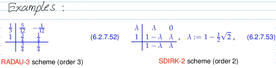
Problem 9-14: Two-Step Radau Runge-Kutta Single-Step Method for the Heat Equation (50 min) "simple" runge-kutta repetition
Problem 9-20: Meithod-of-Lines with SDIRK timestepping (60 min)
in solution for b), shouldn’t the A-matrix integrate over dx instead of dS?
Problem 9-3: Decaying Method-of-Lines Solution with Implicit-Euler Timestepping (130 min)
Week 9 (20.04.-24.04.): 3 h 30 min
Problem 9-17: Scalar Parabolic Evolution Problems: Continuous and Discrete (75 min) similar to 9.14, 9.20 from last week
Problem 9-11: Gauss-Lobatto IIIC Timestepping (135 min) finally a fun programming execise I did understand
preparation: done 2nd time
solution 9.11)g): bottom right matrix block: is there a τ missing?
Week 10 (27.04.-01.05.): 4 h 10 min
Problem 9-21: Magnetic Diffusion in a Wire (210 min)
Problem 12-4: FEM for Stokes BvPs (40 min) important basics
Week 11 (04.05.-08.05.): 7 h 15 min
Problem 12-1: Viscous Flow Simulation with Taylor-Hood FEM (435 min) only Hiptmair and god knew what this problem is about. Now, only Hiptmair knows
this was the most challenging task till now. It takes way longer than 7.5 hours
Week 12 (11.05.-15.05.): 7h 10 min
Problem 10-6: Streamline Upwind Method for Pure Advection Problem (200 min) interesting, nearly succeeded in coding alone -> summary of chapter 2, 10
Problem 12-2: The MINI Element for Stokes (230 min) didn't totally understand b)
in stokesminielement.h, dimension needs to be changed 9x9 -> 11x11 but is not mentioned in solution (error was extremely confusing)
in solution of 12-2)i), the norms for 12.2.27 and 12.2.28 are wrong? ask TA?
13. week (18.05.-22.05.): 7 h 10 min
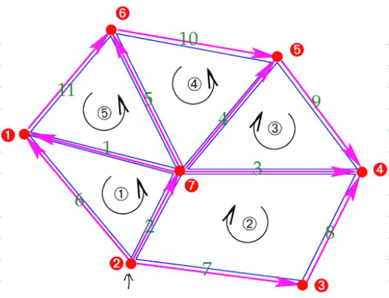
Problem 13-1: Incidence Matrices of a 2D Finite Element Mesh (220 min) didn't understand b), j) fully; mostly copied k) from solution but not overly difficult
wrong code folder: should be IncidenceMatrices, not IncidenceMatricesFEEC
done 2nd time (1.6h)
Problem 13-3: Whitney Finite Elements for Magnetostatic BVP in Two Dimensions (210 min) g) understood everything apart from last flipping lines
14. week (25.05.-29.05.): 6 h 50 min
Problem 13-2: Mixed FEM for the 2D Hodge-Laplacian (410 min) didn't fully understand f), l), o) not sure, took about 7 hours
problem: I don’t understand how to work with HΛ1 / L2Λ1 / L2Λ2, … & vector proxy
in t) / formula 13.2.43 missing supscript 1 on first βj,K1
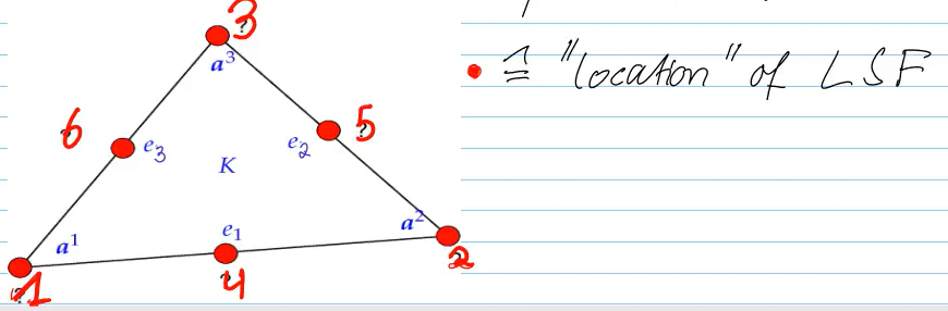
what is LEHRFEM++ numbering for local shape functions [Lecture → § 2.7.4.1] w)?
first those associated with nodes, then edges
Videos
0.0 Welcome and introduction (17min)
week (16.02.-20.02.):
1.2.1 Elastic Membranes (17 min)
1.2.2 Electrostatic Fields (6 min)
1.2.3 Quadratic Minimization Problems (21 min)
1.3 Sobolev spaces (22 min)
1.4 Linear Variational Problems (21 min) didn't quite understand
week (23.02.-27.02.):
1.5 Equilibrium Models: Boundary Value Problems (22 min)
Global shape functions are the elements of the basis of the finite element trial and test space used in step II of a finite-element Galerkin discretization. They are associated with geometric entities of the mesh M and are locally supported. Global shape functions are defined on the whole computational domain Ω. Usually, global shape function will be M-piecewise smooth, but not smooth everywhere.
Local shape functions for a particular cell of the mesh are the (non-trivial) restrictions of global shape functions to that cell. Thus, local shape functions are defined only on a particular cell of the mesh and not beyond. Usually, local shape functions are smooth.
Plugging local shape functions into localized bilinear forms we obtain element matrices.
Vorlesung
1. Second-Order Scalar Elliptic Boundary Value Problems
Video 1.2.1: Elastic Membranes
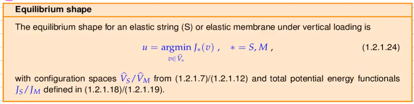
Goal: compute shape of string (1D)/membrane (2D) under vertical loading
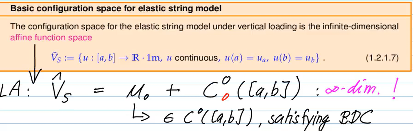
Notion 1.2.1.1. Configuration space
The configuration space of a mathematical model is a set, each of whose elements completely describe all relevant aspects of a state of the modeled physical system.
string must be continuous ⟺ string not ripped apart
b.c.: u(a),u(b) given
-> but need formula for potential energy
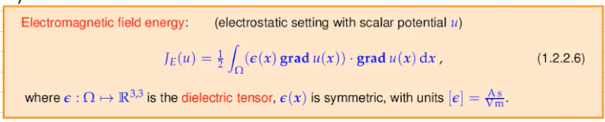
Video 1.2.2 Eloectrostatic Fields (6min)
Note: V^⊂C0(Ω)
Equilibrium condition for electrostatics
The physical field will attain minimal electromagnetic field energy (1.2.2.16)
u∗=u∈VEargminJE(u).
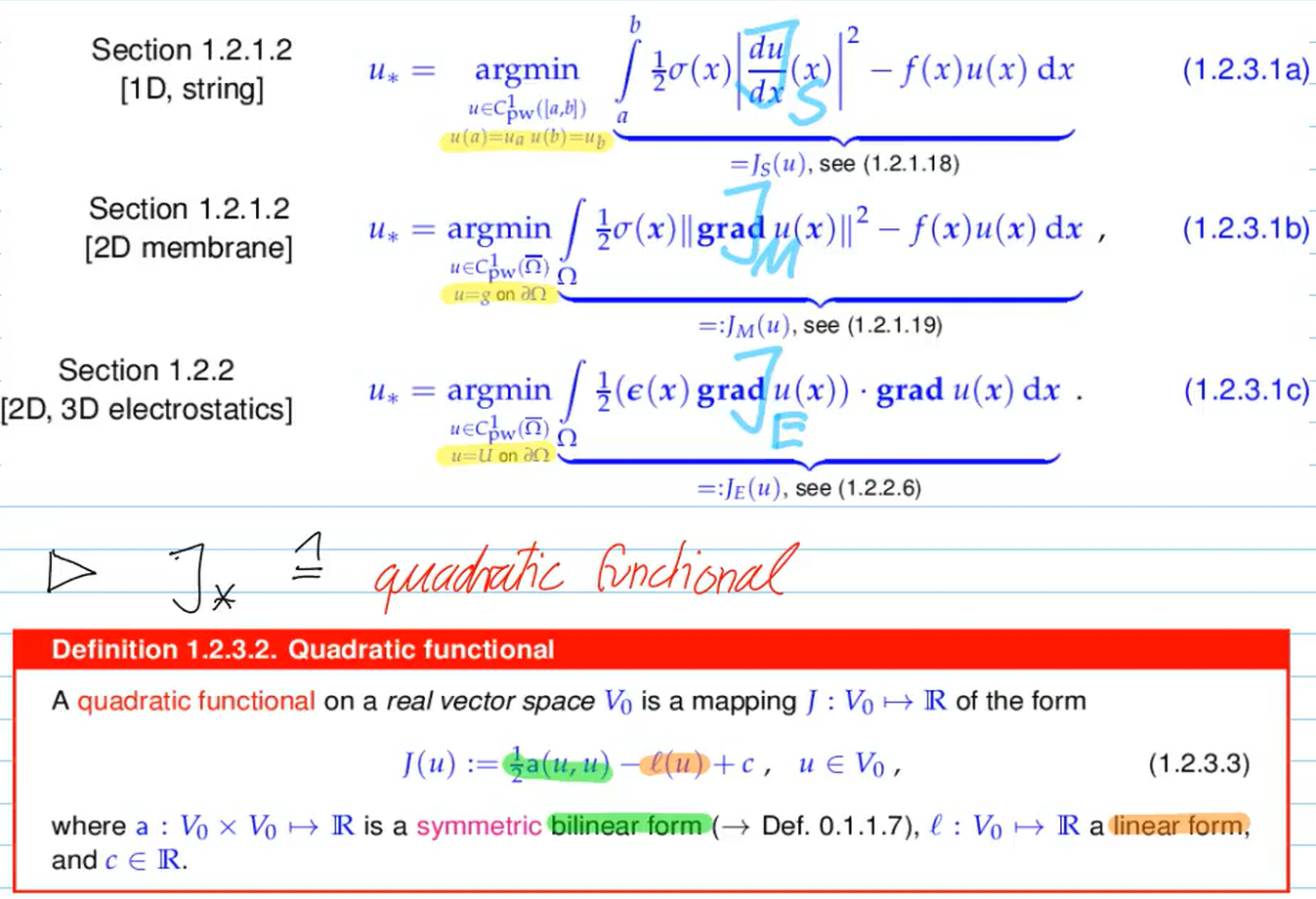
Video 1.2.3 Quadratic Minimization Problems (21 min)
Definition 1.2.3.13. Quadratic minimization problem
A minimization problem
w∗=w∈V0argminJ(w)
is called a quadratic minimization problem, if J is a =quadratic functional on a real vector space V0.
extension to affine space:
V^="offset function"μ0+V0⊂V
Recall from LA:
A=A⊤s.p.d⟹(μ,η)→μ⊤Aη=^inner product
Tldr
we are trying to find the most stable/lowest energy state of the system. The idea is to find a general formula for the structurally similar string/membrane/electricity problem, which can be described by a Quadratic functional:
J(v)=internal energy21a(v,v)−external loadl(v)+c=21x⊤Ax−b⊤x+c(a bilinear + symmetric, l linear)
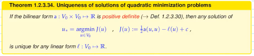
However, we can only solve the problem if the energy formula has a minimum (imagine the energy formula as a paraboloid “bowl”):
Thus, for ∃ of solution, the problem must fulfill:
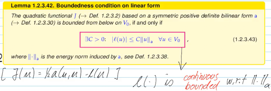
a(v,v)>0∀v=0 -> bilinear form must be at least semi-positive definite
∣l(v)∣≤C∣∣v∣∣a, where ∣∣v∣∣a=a(v,v)energy norm. -> linear form l(v) must be bounded/continuous with respect to energy norm. This ensures the “load” isn’t so strong that it rips the system apart.
have a bad reputation as having a useless mathematical sophistication
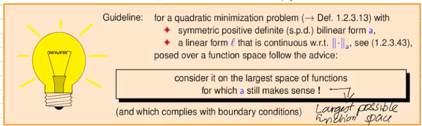
choose
V0:={functions v onΩ:a(v,v)<∞}
=> energy space generated by a(⋅,⋅)
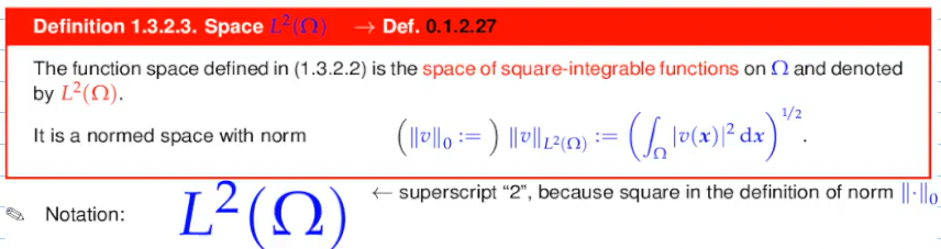
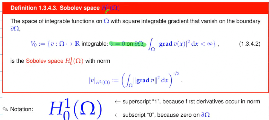
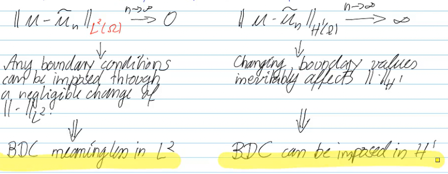
in contrast to L2-Space, here the boundary conditions are not dropped; the reason for this are the norms:
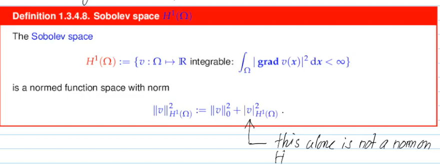
Sobolev space without boundary conditions:
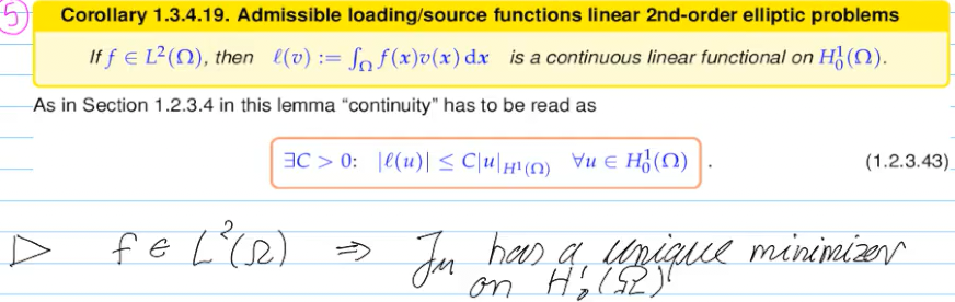
the L2 can be bounded by the size of the domain and the energy norm:
Theorem 1.3.4.17: First Poincaré-Friedrichs inequality
If Ω⊂Rd, d∈N, is bounded, then
∥u∥0≤diam(Ω)∥gradu∥0∀u∈H01(Ω).
⟹∣ℓ(v)∣≤C∥f∥0 diam(Ω)∥v∥a∀v∈H01(Ω)
How to "work with" Sobolev spaces
Most concrete results about Sobolev spaces boil down to relationships between their norms. The spaces themselves remain intangible, but the norms are very concrete and can be computed and manipulated as demonstrated above.
Tip
Do not be afraid of Sobolev spaces!
It is only the norms that matter for us, the ‘spaces’ are irrelevant!
Corollary 1.3.4.26. H1-norm of piecewise smooth functions
Under the assumptions of Thm. 1.3.4.23 we have for a continuous, piecewise smooth functionu∈C0(Ω)
L2 space - space of all functions where ∫f2<∞. Here, b.c. are meaningless, since changing the function at a single point costs zero energy
H1 space - “energy space” for membranes; includes functions where derivatives are square-integrable. Unlike L2, the b.c. cannot be ignored, since changing a point blows up the derivative
H01-space - H1 with zero b.c.
one can think of H1 as the space of peicewise smooth, globally continuous functions
Tldr
Functions of an L2 space are square-integrable on Ω:
∫Ω∣u(x)∣2dx<∞
Functions of the H1 space are in L2, too. Additionally, the first (hence ^1) derivative is in L2, too:
H1(Ω)={u∈L2(Ω)∣∇u∈L2(Ω)}
Note that H1 functions do not need to be in C1 or even C0! A counterexample is
u(x,y)={0,1,x≤21x>21inΩ=[0,1]2
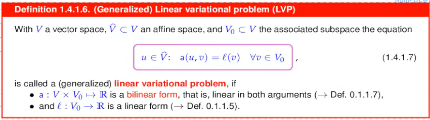
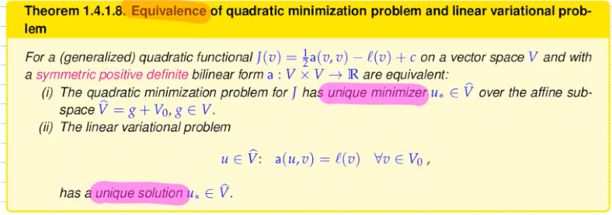
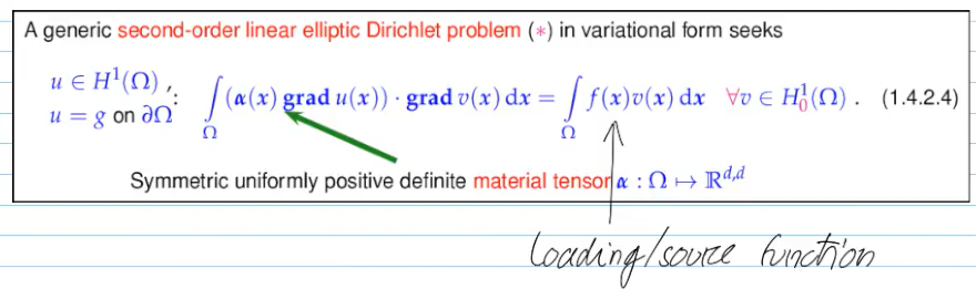
Video 1.4 Linear Variational Problems (21 min)
Poincare-friedrich?
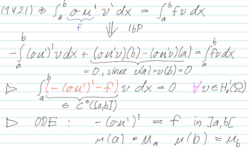
Video 1.5 Equilibrium Models: Boundary Value Problems (22 min)
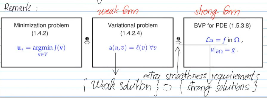
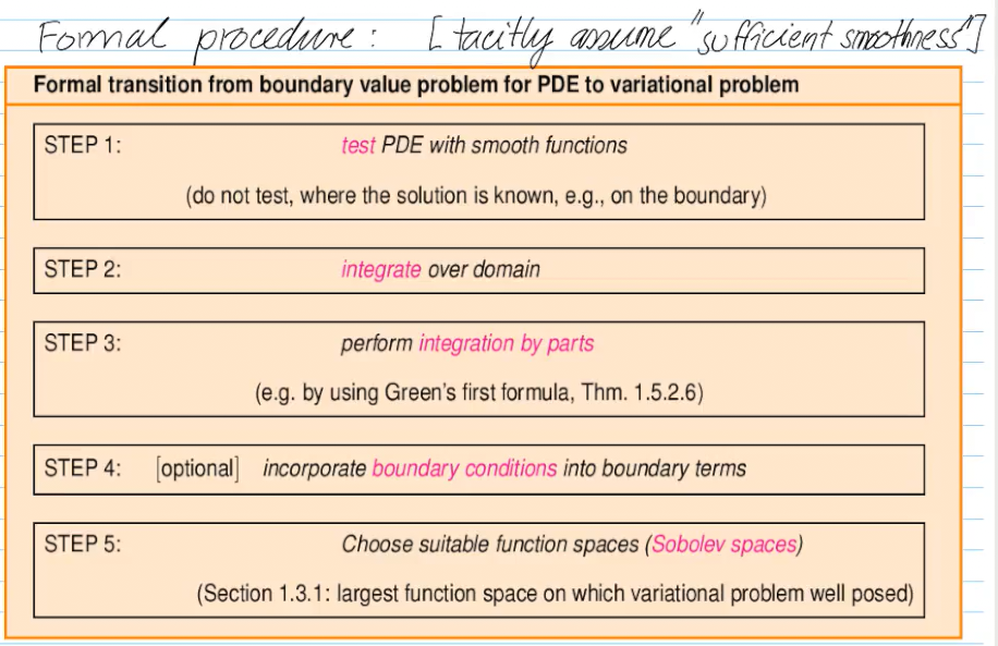
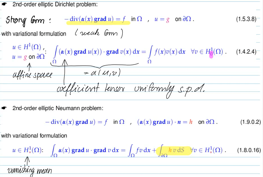
=> 2-pt BVP (a Dirichlet problem) in strong form (vs. “weak form” = LVP)
Lemma 1.5.3.4: Fundamental lemma of calculus of variations in higher dimensions
If f∈L2(Ω) satisfies
∫Ωf(x)v(x)dx=0∀v∈C0∞(Ω),
then f≡0 can be concluded.
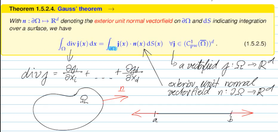
Video 1.6 Diffusion Models: Stationary Heat Conduction (5 min)
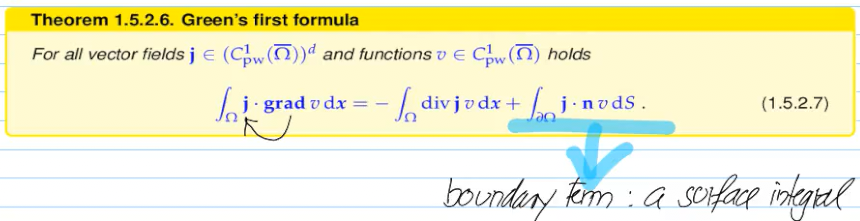
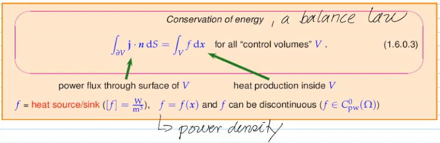
by combining those two using Gauss theorem, we get:
=> we reach at the same PDE as for the membrane model
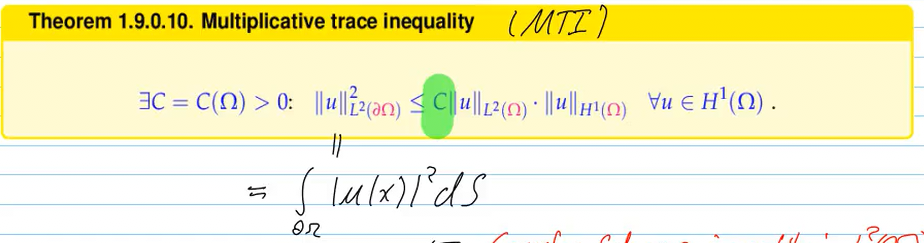
Video 1.7 Boundary Conditions (07.35 min)
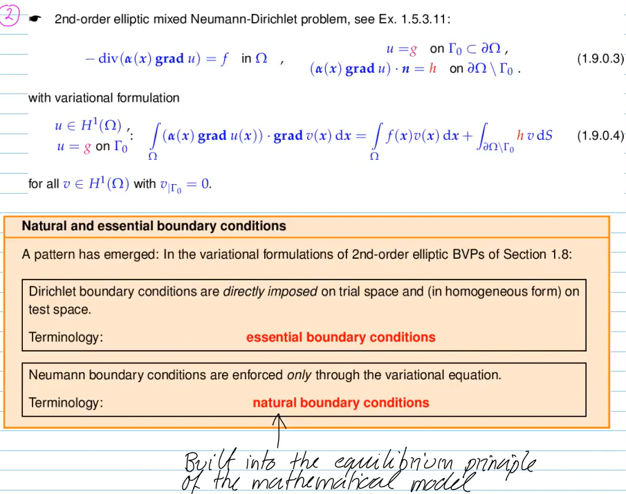
example of a mixed BVP:
Boundary conditions for second-order elliptic BVPs
For second order elliptic boundary value problems exactly one boundary condition is needed on every part of ∂Ω.
Video 1.8 Second-Order Elliptic Variational Problems (13 min)
for Dirichlet BVP:
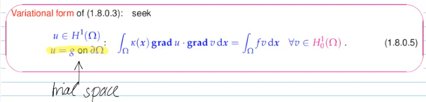
for Radiation BVP:
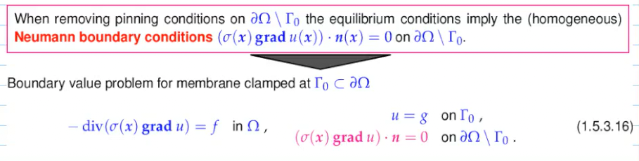
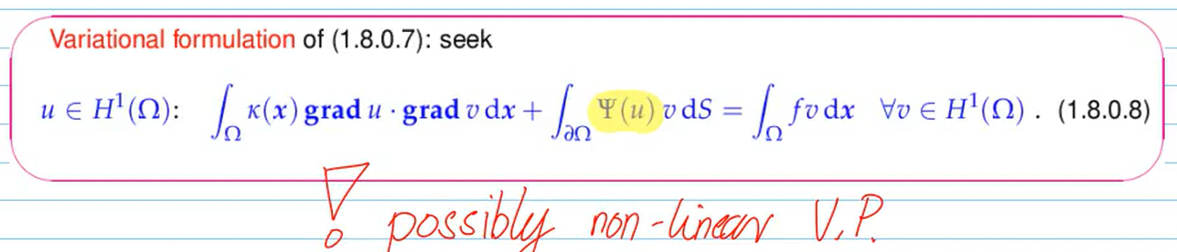
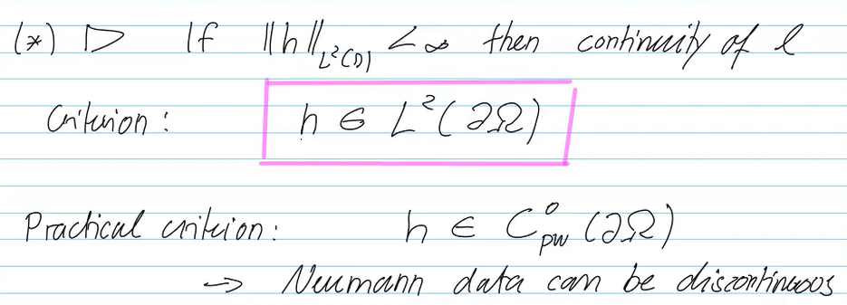
for Neumann BVP:
Theorem 1.8.0.20: Second Poincaré-Friedrichs inequality
If Ω⊂Rd, d∈N, is bounded, then
∃C=C(Ω)>0:∥u∥0≤C diam(Ω)∥gradu∥0∀u∈H∗1(Ω).
Video 1.9 Essential and Natural Boundary Conditions (18 min)
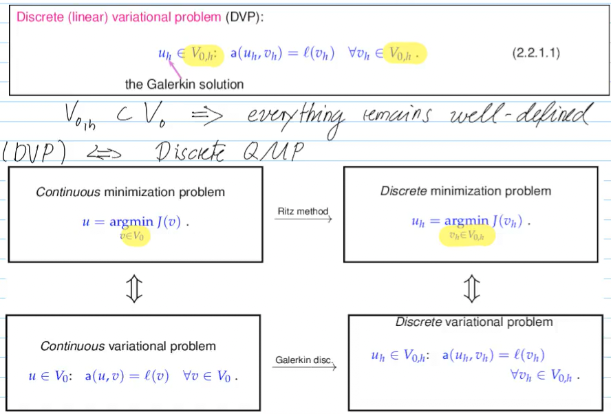
Video 2.2 Principles of Galerkin Discretization (25 min)
graph LR
	A[Variational boundary<br>value problems] -- discretization --> B["System of a finite number of equations for (real) unknowns"]
garlekin discretization in two steps:
V0→V0,h⊂V,dimV0,h<∞
Galerkin discretization (step 1)
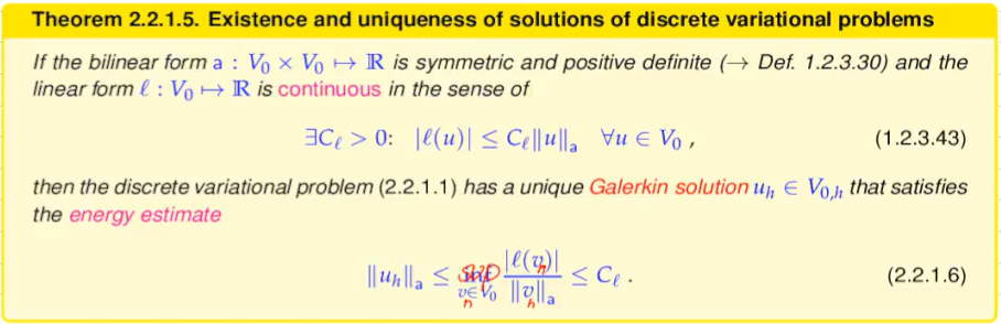
Replace the infinite-dimensional function space V0 in the linear variational problem (2.2.0.2) with a finite-dimensional subspaceV0,h⊂V0.
-> “h” =^ tag for s.th. finite
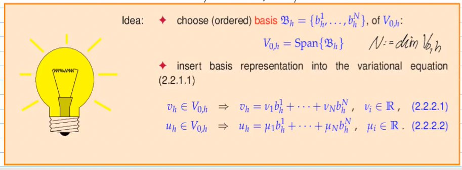
Choose basis, then plug basis expansions int DVP, and use (bi-linearity)
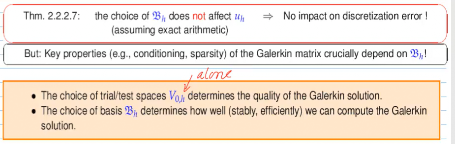
Theorem 2.2.2.7: Independence of Galerkin solution of choice of basis
The choice of the basis Bh has no impact on the (set of) Galerkin solutions uh of (2.2.1.1).
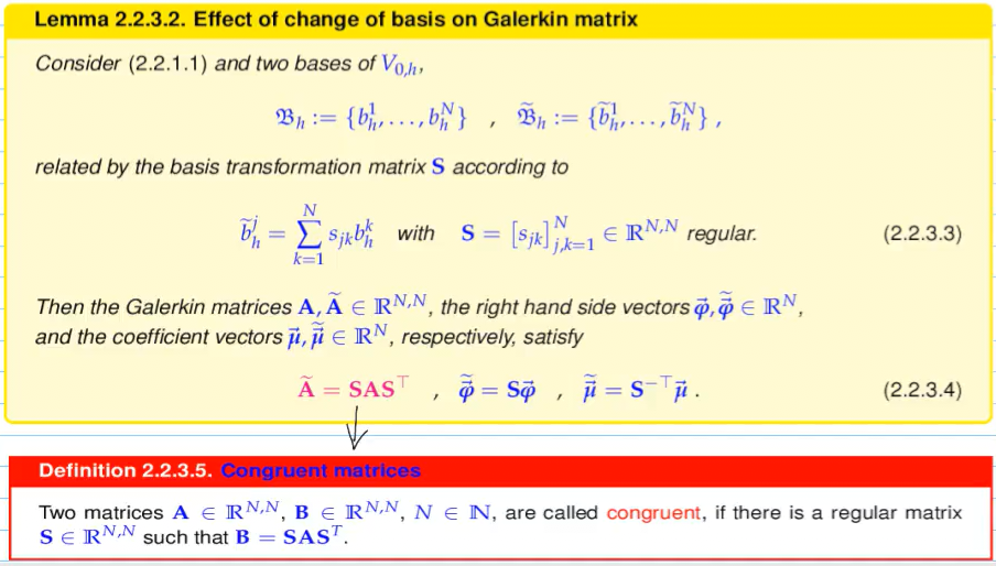
Properties all Garlekin matrices for a DVP (all matrices from a congruence clas) share:
regularity (invertibility)
symmetry
pos.dev.
Garleking pos. dev / symm.⟺a(⋅,⋅)s.p.d onV0,h
Video 2.3 Case Study: Linear FEMfor Two-Point Boundary Value Problems (24 min)
u′′=fin[a,b]u(a)=u(b)=0
NOTE: f∈L2(Ω)is given inprocedural form, f∈C0([a,b])
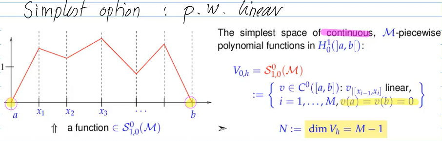
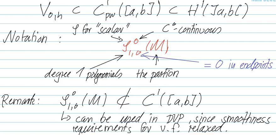
Idea underlying the finite element method: approximate u by means of continuous, piecewise polynomial functions on a mesh:
Video 2.4 Case Study: Triangular Linear FEMin Two Dimensions I (28 min)
In 1D, we partition the domain Ω into an 1D Mesh
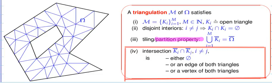
In 2D, we use triangulation
4. means: no hanging nodes (nodes that are on the edge of another triangle)
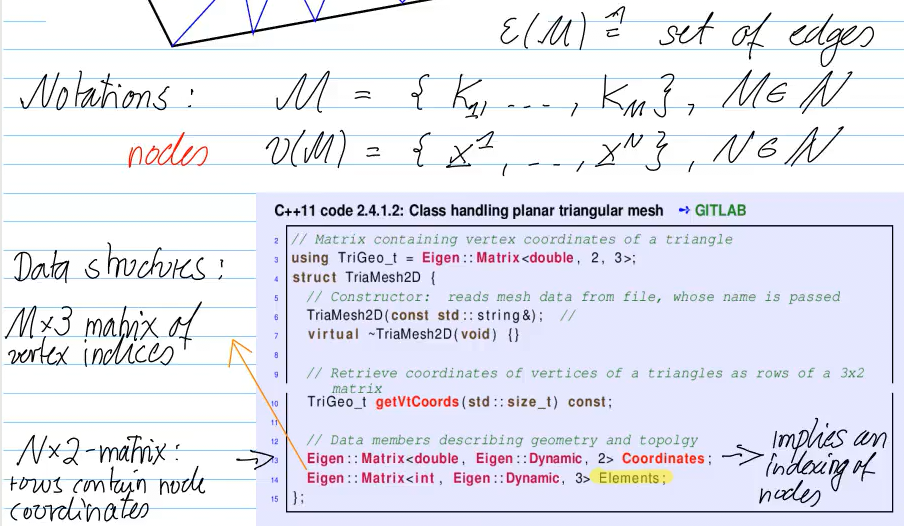
ϵ(M)= set of edges
M={K1,…,KM},M∈N
v(M)={x1,…,xN},N∈N
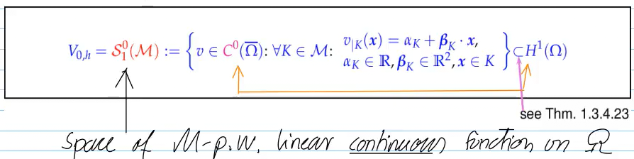
test space in 2 (space of M-p.w. linear continuous function on Ω):
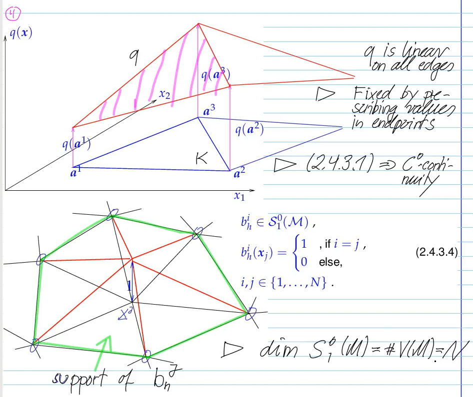
tent function alternative in 2D:
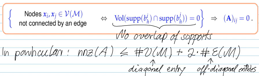
In 2D, the Galerking matrix does not have a nice structure like in 1D; however, it is still sparse, since nodes unconnected by edges result in a 0 in the Matrix:
Video 2.4 Case Study: Triangular Linear FEMin Two Dimensions II (32 min)
Galerkin discretization based on a nodal basis of tent functions and a triangular mesh:
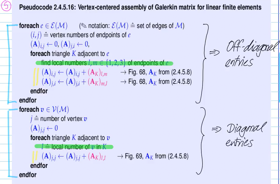
there are two approaches to creating the Galerkin-matrix:
assemble matrix from all vertices
Problems:
Edges not available in data structure (see first 2.4 video)
Triangles adjacent to nodes not available
In my opinion, it is not fair to compare it with the cell-oriented approach, when the data class is also cell-oriented
cell-oriented approach, by “distribute & add”
for finite-element algorithms, always do it cell-oriented
dof: degrees of freedom
now, we assemble everything:
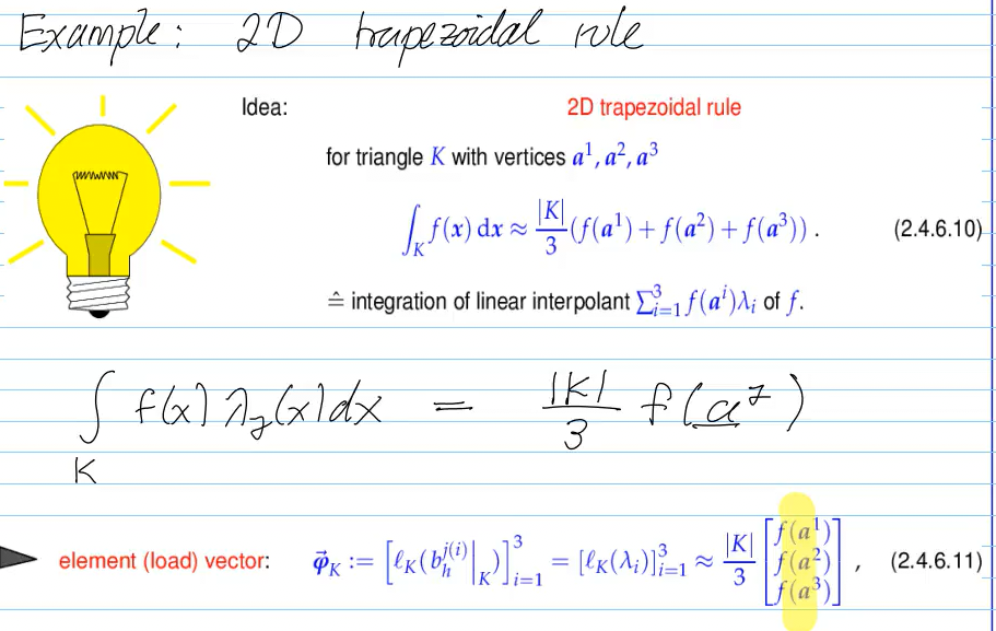
for the RHS, we can compute the integral using composite trapezoidal rule (we are working with triangles anyways):
Tldr
We are trying to get variational problems from infinite-dimensional function spaces to something discrete by
choosing a finite-dimensional subspaceV0,h⊂V0, where the bilinear and linear form a(⋅,⋅),l(⋅) remain well-defined
choosing an ordered basis{b1,…,bN} for the subspace V0,h,dim(V0,h)=N, and using the basis to convert problem into a linear system
In those two steps, the problem can be transformed into a LSE
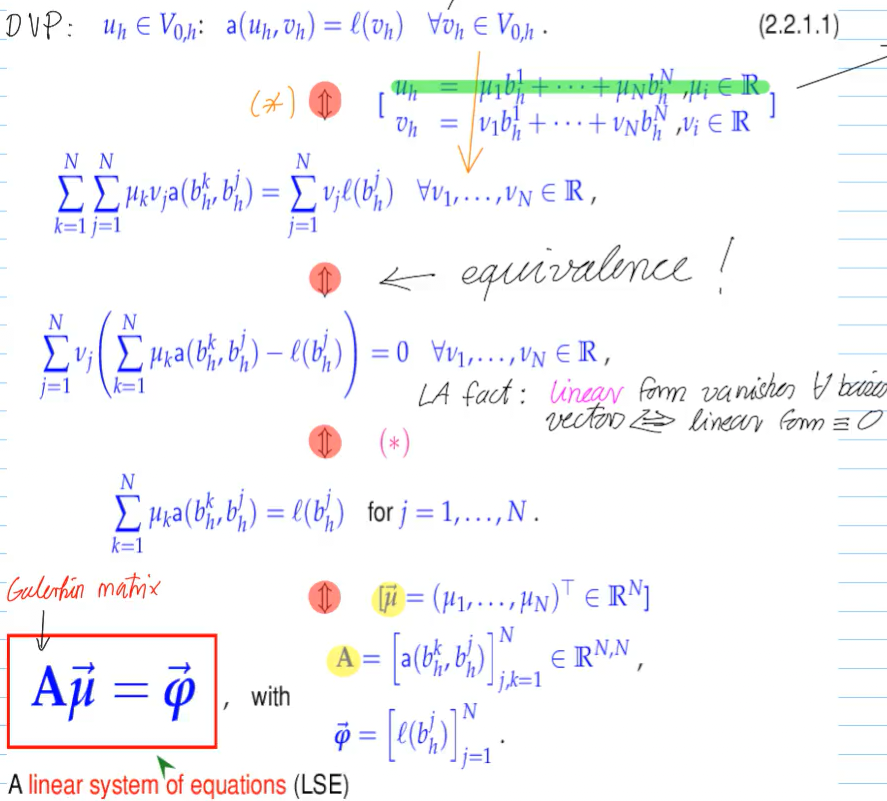
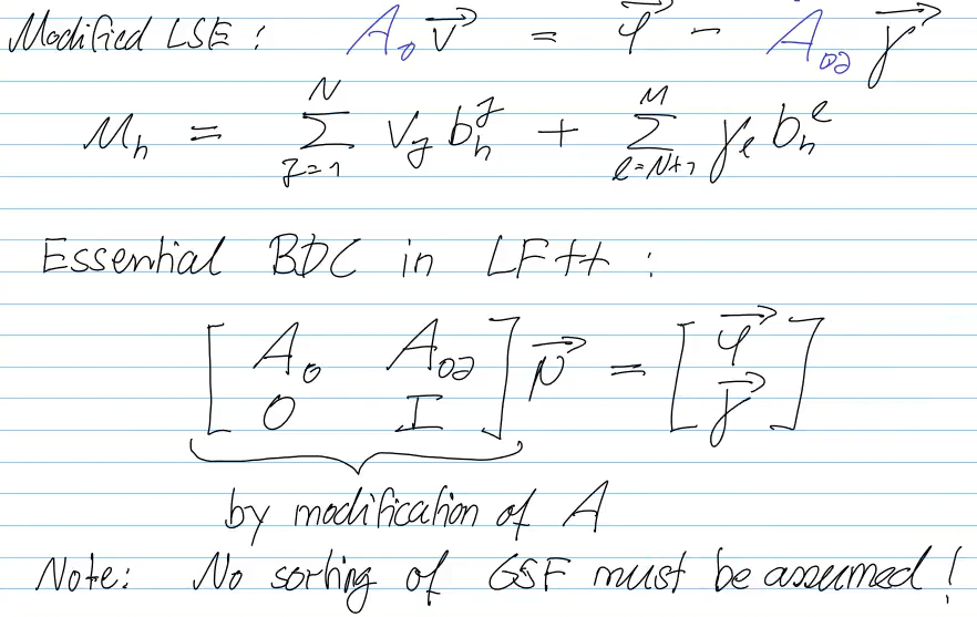
Aμ=ϕ
Tldr - Step 1
In the first step of the discretization, our goal is to replace space V0,dim(V0)=∞ with finite V0,h⊂V0. The space should preserve the bilinear form a(⋅,⋅) and linear form l(⋅). The new problem is:
finduh∈V0,hs.t.a(uh,vh)=l(vh)∀vh∈V0,h
define Mesh M. Normally, we use triangulation - pay attention that the mesh does not have “hanging nodes” (2.4.1)
choose a “building block” function to use for each cell. Normally, pecewise linear functions are used, evtl. quadratic or cubic polynomials
ensure C0 -> do not use piecewise constants, since then V0,h⊂V0, e.g. if V0=H1
incoroporate boundary conditions, in case of Dirichlet by discarding any basis functions with nodes on the boundary
Tldr - Step 2
choose a basis Bh={b1h,…,bNh}, then write every vh∈V0,h as linear combination of basis functions:
uh=j=1∑Nμjbjh,vh=i=1∑Nνibih
convert to a linear system by exploiting bilinearity of a(⋅,⋅) and linearity of l(⋅):
j=1∑Nμja(bjh,bih)=l(bih)fori=1,…,N⟺Aμ=ϕ
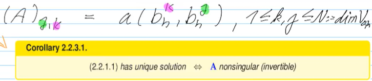
A: Galerkin/stiffness matrix, Aij=a(bjh,bih), how basis functions interact through the bilinear form
ϕ: load vector, ϕi=l(bih)
μ: solution vector; the final Galerkin solution uh=∑bih⋅μi (basis, weighted by solution vector)
Basis choice
no impact on Galerking solution; however:
basis functions with small local support (e.g. tent function) results in a sparse matrix -> desired outcome
basis choice determines condition number of matrix -> sensitivity to rounding errors
Video 2.5 Building Blocks of General Finite Element Methods (22 min)
Lemma 2.5.2.8: Dimension of spaces of tensor product polynomials
dimQp(Rd)=(p+1)dfor all p∈N0,d∈N
2nd option: e.g.
Q2(R2)=span⎩⎨⎧1,x,x2y,yx,yx2y2,y2x,y2x2⎭⎬⎫
basis functions (also called global shape functions (GSF), degrees of freedom)
Locally supported basis functions
Third main ingredient of FEM: locally supported basis functions (see Section 2.2 for role of bases in Galerkin discretization)
Basis functions bh1,…,bhN for a finite element trial/test space V0,h built on a mesh Mmust satisfy:
(B1) Bh:={bh1,…,bhN} is basis of V0,h⟹N=dimV0,h,
(B2) each bhi is associated with a single geometric entity (cell/edge/face/vertex) of M,
(B3) supp(bhi)=⋃{K:K∈M,p⊂K}, if bhi associated with cell/edge/face/vertex p.
we want local support:
if supp(bhi), supp(bhj) don’t overlap, entries in Galerkin matrix (A)ij=0 => sparse matrix
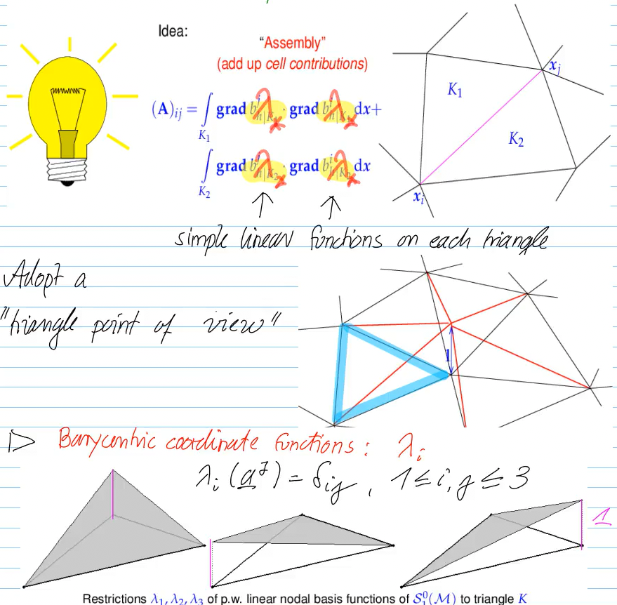
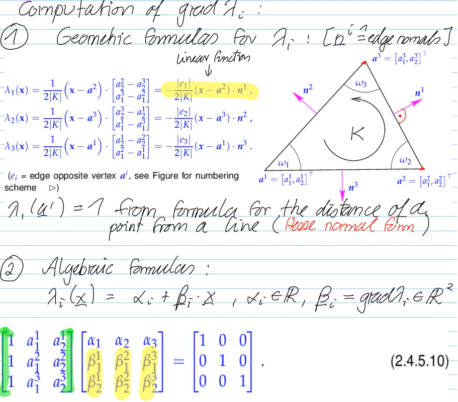
generalization of barycentric coordinate functions:
Video 2.6 Lagrangian Finite Element Methods (23 min)
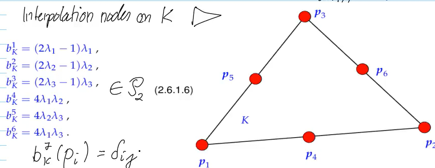
one triangle, with Kardinal property:
gluing triangles (interpolation nodes):
-> globally continuous piecewise function
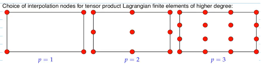
for more dimensions, we “subdivide”; then, we might also have interpolation nodes inside the shape
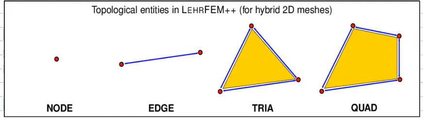
for hybrid mesh:
works, becuase functions ∈Q1/P1 are all linear when restricted to straigt edge (which we have)
works for any degree!
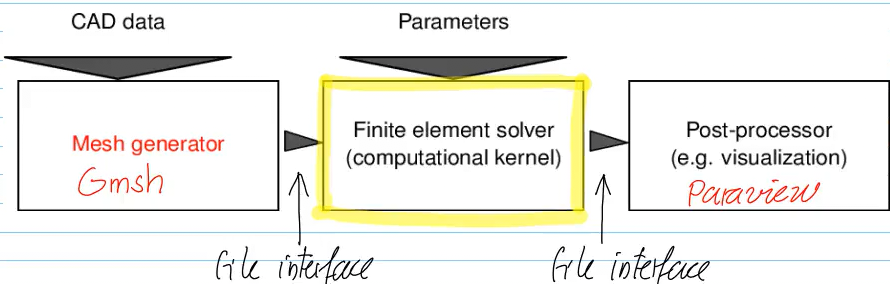
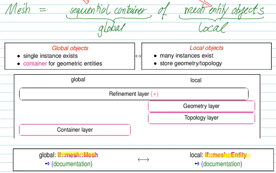
Video 2.7.2 Mesh Information and Mesh Data Structures (21 min)
problems with FEM:
// factory object creates mesg entities auto of 2D mesh data structure from information contained in mesh_fileauto factory = std::make_unique<lf::mesg::hybrid2d::MeshFactory>(2);lf::io::GmshReader reader(std::move(factory), mesh_file.string());
we need
container (tranversal + ordering/indexing of entities)
in 1D: affine mapping [a,b]→[−1,1] + transformation formula for integrals
local quadrature rules used in finite element methods are botained by transformation from (a few) local quadrature rules defined on reference elements.
in 2D:
(affine mapping maps lines to lines)
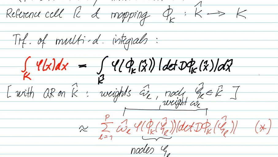
general formula:
example on K∈M:
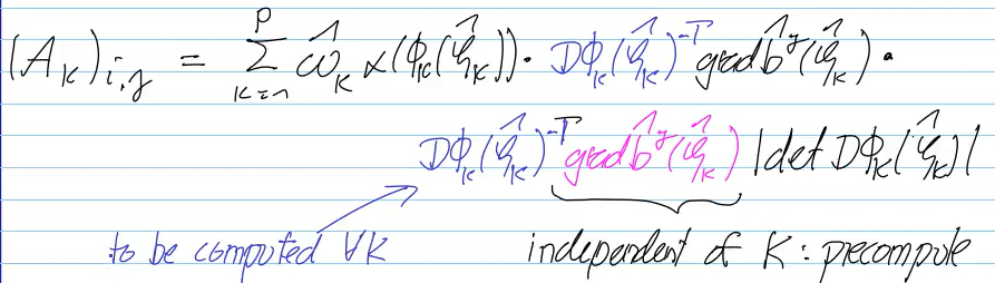
however, if ϕK affine => det(DϕK)≡const., and we get:
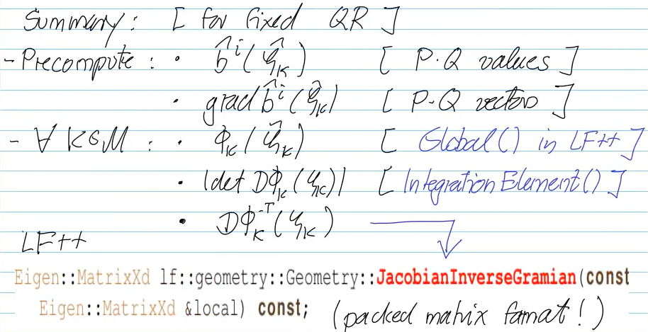
in LehrFEM, we can use:
Definition 2.7.5.29: Order of a local quadrature rule
A local quadrature rule according to Def. 2.7.5.9 is said to be orderq∈N, if
for a simplex K (triangle, tetrahedron) it is exact for all polynomialsf∈Pq−1(Rd),
for a tensor product element K (rectangle, brick) it is exact for all tensor product polynomialsf∈Qq−1(Rd).
“order ↑⟹ no. of nodes ↑”
transformation on affine maps preserves polynomials
-> integral transformation doesn’t change order of polynomials
quadrature rules in LehrFEM: reference object shape + desired order
not copied: code 2.7.5.41: Entity-based composite numerical quadrature
Video 2.7.6 Treatment of Essential Boundary Conditions (21 min)
gluing:
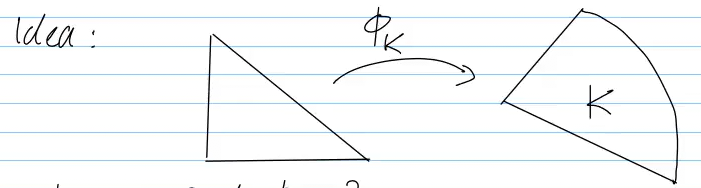
-> local shape functions are no longer bilinear, since ϕK−1 is no longer polynomial (rational function)
Non-polynomial nature of bilinear shape functions
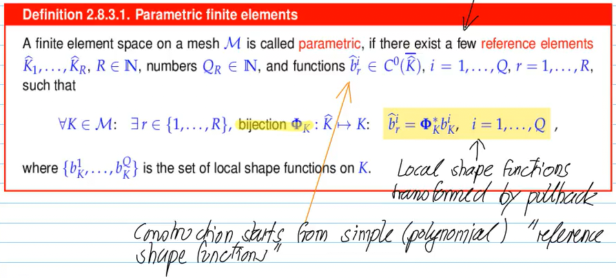
The local shape functions bKi defined by (2.8.2.4), where ΦK is a bilinear transformation and bi are the bilinear local shape functions on the unit square, are not polynomial in general.
Video2.8 Parametric Finite Element Methods II (27 min)
Note that possibility of gluing needs to be checked!
-> As regards the energy norm, the Galerkin solution is the best possible solution we can obtain in a given trial space.
Galerking error estimates in energy form approximation error estimates
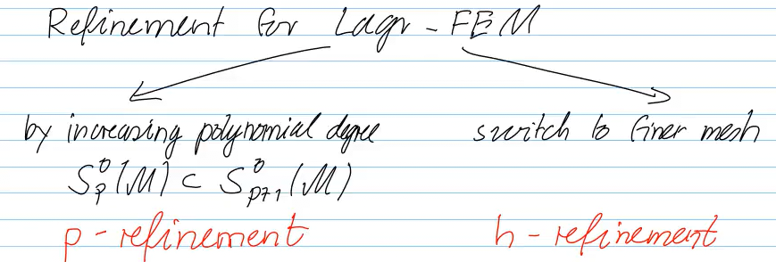
we can improve the result by enlarging the space (refinement)
2d triangular: regular refinement by splitting triangle into 4 congruent triangles
use lf::refinement in LF++
Video 3.2 Empirical (Asymptotic) Convergence of Lagrangian FEM (26 min)
Asymptotic Convergence
Convergence: asymptotic perspective
Crucial: our notion of convergence is asymptotic!
sequence of discrete models ⟹ sequence of approximate solutions (uh(i))i∈N↕⟹ study sequence (∥uh(i)−u∥)i∈N as $i \to \infty$
created by variation of a discretization parameter.
Definition 3.2.1.4. Mesh width
Given a mesh M={K}, its mesh width $h_{\mathcal{M}}$ is defined as
hM:=max{diamK:K∈M},diamK:=max{∣p−q∣:p,q∈K}.
limit hm -> 0
for p-refinement, discretication DP =^ degree p
cost might depend on dimension V0,h (or nnz(A))
algebraic and exponential convergence
Definition 3.2.2.1. Types of convergence → ,
∥u−uN∥∥u−uN∥=O(N−α),α>0=O(exp(−γNδ)), with γ,δ>0⟺algebraic convergence with rateα⟺exponential convergence
(asymptotically for N→∞)
log-log plot with straigt line: algebraic convergence
lin-log plor with line: exponential convergence
-> (integral) error norms can usually be computed only by numerical quadrature (/sampling) of sufficiently high order
Example:
alg. cvg., but slow convergence for non-smooth solutions (h-refinement)
L2 cvg. seems to be faster than ∥⋅∥a-cvg (?)
exp. cvg.(p-refinement)
-> there might be pre-asymptotic behaviour (no convergence until mesh fine / polynomial degree high)
Tldr: h- vs p- refinement
Feature
h-Refinement
p-Refinement
Strategy
Subdivide mesh cells (h→0)
Increase local polynomial degree (p→∞)
Typical Convergence
Algebraic: O(hp)
Exponential: O(exp(−γpδ)) for analytic solutions
Limiting Factor
Polynomial degree p and smoothness k
Smoothness k of the exact solution
Space Property
Often results in nested spaces (e.g., via regular refinement)
Inherently leads to nested finite element spaces
Video 3.3 A Priori (Asymptotic) Finite Element Error Estimates I (10 min)
“How many derivatives must a function have (in a weak, square-integrable sense) before we can guarantee it is actually a continuous, point-wise defined function?”
e.g. d=2: m>1 => H2(Ω) functions are guaranteed to be continuous
Video 3.3 A Priori (Asymptotic) Finite Element Error Estimates III (16 min)
Theorem 3.3.5.6. Best approximation error estimates for Lagrangian finite elements
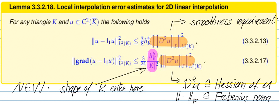
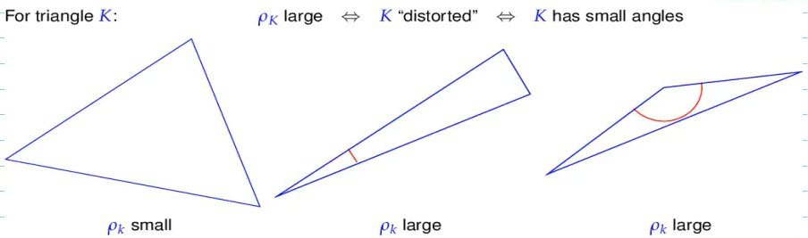
Let Ω⊂Rd,d=1,2,3, be a bounded polygonal/polyhedral domain equipped with a mesh M consisting of simplices or parallelepipeds. Then, for each k∈N, there is a constant $C > 0$ depending only on $k$ and the shape regularity measure $\rho_{\mathcal{M}}$ such that
=> Algebraic convergence of discretization error with respect to N (DOFs), rate
d1min(p,k−1)
rate limited by
polynomial degree p
smoothness
rate deteriorates for larger d
By what extra cost can we buy a certain improvement of the FEM solution? (3.3.5.23)
Assuming the a priori error estimate is sharp (the actual error follows the theoretical trend), the relationship between error reduction and computational cost is:
The Goal (Gain): Reduce the discretization error (energy norm) by a factor of ρ>1.
The Price (Cost): Increase the number of unknowns (N) by a factor of:
Cost Factor≈ρminp,k−1d
takeaways
The Curse of Dimension (d): As the spatial dimension d increases, the cost of reducing error grows exponentially. Accuracy is much “cheaper” in 1D than in 3D.
Optimal Efficiency (p=k−1): For best gain/cost, polynomial degree p should match solution’s smoothness k (Hk)
Smoothness Matters: For very smooth solutions (k is large), high-order elements (p>1) reduce the required increase in N significantly compared to linear elements (p=1).
The “Slow” Limit: If the solution is not smooth (small k), increasing the polynomial degree p does not help efficiency, because the cost factor will be stuck at ρd/(k−1) regardless of how high you choose p.
type of refinement
alg. cvg. rate
h-refinement (p fixed & small: p≤k−1)
−p/d
h-refinement (low regularity of u: k≤p+1)
−(k−1)/d
p-refinement (hm fixed, limited regularity u)
−(k−1)/d
p-refinement (perfectly smooth (analytic) solution) (because C depends on k in unspecified way)
theorem doesn’t work
Here is a compressed summary of Unit 3.3 for your markdown callout, based on the course videos and documents:
Tldr 3.3: A Priori Finite Element Error Estimates
Cea’s Lemma: energy norm of discretization =^ best approximation error of FE space
accuracy is governed by the mesh width (hM), the polynomial degree (p), and the Sobolev smoothness (u∈Hk) of the exact solution.
where the generic constant C depends on the shape regularity (ρM) of the mesh but is independent of hM.
Algebraic Convergence Trends (h-refinement): On quasi-uniform meshes, the error decays relative to the number of unknowns (N) as:
Error Norm(N)≈CN−α,with rate α=dmin{p,k−1}
Curse of Dimension: Convergence speed deteriorates as the spatial dimension d increases.
Rate Limits: The rate is limited by either the polynomial degree p (for smooth solutions) or the solution’s lack of regularity k (for rough solutions).
Asymptotic Efficiency (Cost-Benefit): Reducing the error by a factor ρ>1 requires increasing the problem size N by a factor of ρd/minp,k−1. Efficiency is theoretically optimal when p=k−1.
todo Learn more about Sobolev regularity (solution u⊂Hk(Ω), which k?)
Video 3.4 Elliptic Regularity Theory (11 min)
WHat is the Sobolev regularity of solutions of elliptic BVP?
Theorem 3.4.0.2. Smooth elliptic lifting theorem
If ∂Ω is C∞-smooth, ie. possesses a local parameterization by C∞-functions, and σ∈C∞(Ω), then, for any k∈N,
In addition, for such u there is C=C(k,Ω,σ) such that
∥u∥Hk+2(Ω)≤C∥div(σgradu)∥Hk(Ω)
probably irrelevant:
Theorem 3.4.0.6. Corner singular function decomposition
Let Ω⊂R2 be a polygon with J corners ci. Denote the polar coordinates in the corner ci by (ri,φi) and the inner angle at the corner ci by ωi. Additionally, let f∈Hl(Ω) with l∈N0 and l=λik−1, where the λik are given by the singular exponents
λik=ωikπfor k∈N.(3.4.0.7)
Then u∈H01(Ω) with =−Δu=f= in Ω (Dirichlet prob.) can be decomposed
Ω⊂R2 has re-entrant corners⟹ if u solves Δu=f in Ω, u=0 on ∂Ω, then u∈/H2(Ω) in general.
however, for convex problems, the dirichlet solution is in H2 (BVP is 2-regular)
Theorem 3.4.0.10. Elliptic lifting theorem on convex domains
If Ω⊂Rdconvex, u∈H01(Ω),Δu∈L2(Ω)⇒u∈H2(Ω).
Video 3.5 Variational Crimes (15 min)
“theory is incredibly difficult”
Variational crime: instead of solving exact discrete variational problem, we solve a perturbed one:
ah(u~h,vh)=lh(vh)
-> inevitable, since some functions are only given in procedural form
Guideline for acceptable variational crimes
Variational crimes must not affect (type and rate) of asymptotic convergence
Impact of Numerical Quadrature
Note: To show that QR is of order 2 -> show that it integrates polybomials of order 1 exactly (n-1) -> integrates λ1,λ2,λ3 exactly
Intermediate
Finite element theory tells us that the above guideline can be met, if the local numerical quadrature rule has sufficiently high order. The quantitative results can be condensed into the following rules of thumb:
Target Accuracy
Required Quadrature Order
∥u−uh∥1=O(hMp)
Order 2p−1 sufficient for fh
∥u−uh∥1=O(hMp)
Order 2p−1 sufficient for ah
Example of crime: Using midpoint rule (order 2) for quadratic elements (p=2) will cause convergence rate in terms of N to drop.
Impact of boundary approximation
Rule of thumb deduced from sophisticated finite element theory:
If V0,h=Sp0(M), use boundary fitting with polynomials of degree p.
for quadratic FEM, use quadratic boundary approximation (see chapter 2)
Example of crime: When Ω has curved boundary, approximation with polygon (linear) is a crime (perturbed domain Ωh)
When using LehrFEM to refine meshes, the boundary stays the same -> round boundary does not get "rounded" when refining
Video 3.8 Validation and Debugging of Finite Element Codes (13 min)
matching theoretical rates are a strong circumstatial evidence of correctness
-> if code converges mroe slowly than theory predicts, there is almost certainly a bug
3 main methods:
observing convergence between mesh levels
test code by comparing solutions on a sequence of nested meshes created by regular refinement
refine mesh -> ∣uk−uk−1∣ should shrink
norm of the difference, ∣∣uk−uk−1∣∣ should display the same algebraic convergence rate (α) as the actual discretization error
shortcut: compare the difference of their norms (∣∣∣uk∣∣−∣∣uk−1∣∣∣), should also converge at rate α
method of manufactured solutions
most popular way to test a solver
Step 1: Pick a simple domain and a smooth analytic functionu to be your “exact solution”.
Step 2: Use the strong form of the PDE to symbolically calculate what the source function f and boundary data g must be to produce that solution u.
Step 3: Run your solver with this “manufactured” f and g and measure the error ∣∣u−uh∣∣ using overkill quadrature.
Debugging: Plot the error on a log-log scale. If the slope (rate) is wrong, simplify the problem—for example, set the reaction coefficient γ to zero to see if the bug is in the stiffness matrix or the mass matrix.
Direct Testing of Bilinear Forms
test specific parts of your code, e.g. Galerkin matrix for a specific boundary term
Pick a smooth function w and compute the value of the bilinear form b(w,w)analytically using a tool like Mathematica.
-> difference between the analytical value and the discrete value should converge at the polynomial degree rate P as the mesh is refined.
Warning
Avoid polynomial solution: polynomial as manufactured solution will have 0 error -> no convergence rate
Smothness matters: singularities in the solution can “foil” the fast convergence you expect to see
9. Second-Order Linear Evolution Problems
Video 9.2.1 Heat Equation (10 min)
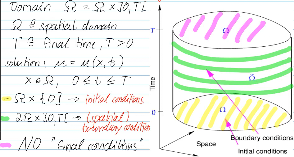
linear evolution: time-dependent / transient
posed on space-time cylinder
9.2 Parabolic Initial-Boundary Value Problems
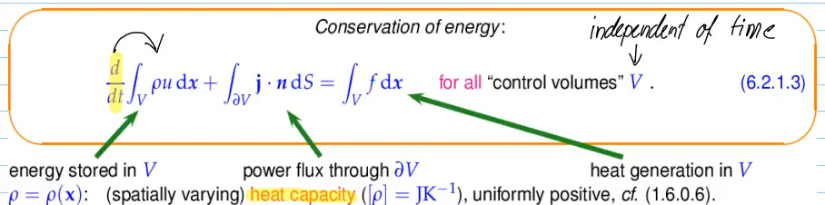
balance law:
using localization and fourier law, we get:
∂t∂(ρu)−div(κ(x)gradu)=finΩ~:=Ω×]0,T[
spatial b.c.:
For second order parabolic evolutions we can/must use the same spatial boundary conditions as for stationary second order elliptic boundary value problems
(although the boundary conditions are now dependent from x and t)
since s.p.d., can be invertedy -> use Cholesky-decomposition ( todo what is that?)
MOL-ODE is stiff!
Explicit Euler timestepping is not stable (exponential blow-up) in case of large timestep combined with fine mesh.
Lemma 6.2.7.32. Behavior of generalized eigenvalues
Let M be a simplicial mesh and A, M denote the Galerkin matrices for the bilinear forms a(u,v)=∫Ωgradu⋅gradvdx and m(u,v)=∫Ωu(x)v(x)dx, respectively, and V0,h:=Sp,00(M). Then the smallest and largest generalized eigenvalues of Aμ=λMμ, denoted by λmin and λmax, satisfy
diam(Ω)21≤λmin≤C,λmax≥ChM−2,
where the “generic constants” (→ Rem. 3.3.5.10) depend only on the polynomial degree p, the domain Ω, and the shape regularity measure ρM.
-> timestep constraint: τ≤Chm2 (similar to ode45)
diagonalization of RK-SSM (φ≡0)
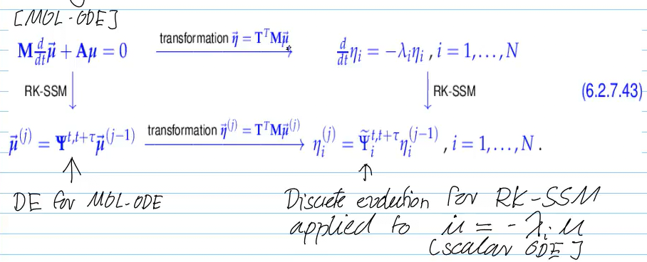
Unconditional stability of single step methods
Necessary condition for universal unconditional stability of a single step method for semi-discrete parabolic evolution problem (7.1.4.4) (“method of lines”):
The discrete evolution Ψλτ:R↦R of the single step method applied to the scalar ODE u˙=−λu satisfies
λ>0⟹j→∞lim(Ψλτ)ju0=0∀u0∈R,∀τ>0.(6.2.7.45)
RK-SSM for u˙=−λu⇒u(j)=stability functionsS(−λτ)u(j−1)
RK-SSM is unconditionally stable for MOL-ODE if ∣S(z)∣≤1∀z<0
evne desirable ∣S(z)∣≪1 for z<0
Definition 6.2.7.48. L( π)-stability
A Runge-Kutta single-step method satisfying (7.1.7.45) is called L(π)-stable, if its stability function S(z) according to (7.1.7.47b) satisfies
∣S(z)∣<1 for all z<0, and
"S(−∞)" :=limz∈R→−∞S(z)=0.
necessarily implicit
Video 9.2.8 Fully Discrete Method of Lines: Convergence (18 min)
The Parabolic Discretization Path
Heat Equation (Strong Form): transient heat equation on a space-time cylinder Ω×]0,T[, subject to initial and boundary conditions:
∂t∂u−Δu=f(x,t)in Ω,u(x,t)=0on ∂Ω
Spatial Variational Formulation: By treating time t as a passive parameter and applying integration by parts in the spatial domain, the PDE is converted to a weak form:
Abstract Formulation: The weak form is generalized into an abstract parabolic evolution problem using the mass bilinear form m(⋅,⋅) and the stiffness bilinear form a(⋅,⋅):
m(u˙,v)+a(u,v)=ℓ(t)(v)∀v∈V0
Method of Lines ODE: Applying Galerkin discretization in space (e.g., using finite elements) transforms the abstract evolution into a system of ordinary differential equations for the coefficient vector μ(t):
Mμ˙(t)+Aμ(t)=φ(t)
where M is the mass matrix and A is the stiffness matrix.
5. Runge-Kutta Method (Full Discretization): Finally, the semi-discrete ODE is integrated in time using a single-step method (SSM). For parabolic problems, L-stable Runge-Kutta methods (such as Radau methods) are preferred to ensure stability:
μ(j)=Ψτ,tj−1μ(j−1)
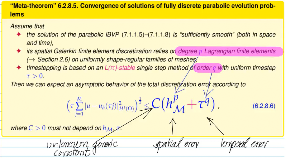
resulting in a fully discrete scheme where the total error is the combined effect of spatial and temporal discretization.
Refinement for fully discrete parabolic evolution problems
Guideline: spatial and temporal resolution have to be adjusted in tandem
for a conditionally stable explicit method, we often have timestep constraint τ≤Ch2
-> if we reduce mesh for accuracy, we have to reduce the timestep more severly than accuarcy requires -> inefficiency “overkill constraint”
-> use unconditionally stable implicit methods instead
10. Modeling Fluid Flow
Video 10.1.1 Modeling Fluid Flow (7 min)
flow field v:Ω→Rd=^ velocity field
needs to be at least Lipschitz-continuous
if v⋅n=0 -> no in/outflow -> streamlines exists for all times
streamline ODE
y˙=v(y)
flow map
Φ:{R×Ω⟶Ω(t,y0)⟶Φty0:=y(t)
where t↦y(t) solves IVP for streamline with y(0)=y0
properties:
Φ0y0Φs+t=y0∀y0∈Ω=Φs∘Φt
Video 10.1.2 Heat Convection and Diffusion (5 min)
where det:Rn,n→R is the matrix determinant and tr stands for the trace of a matrix.
Theorem 10.1.3.8. Divergence-free velocity fields for incompressible flows
A stationary fluid flow in Ω⊂Rd is incompressible (→ Def. 10.1.3.1), if and only if its associated velocity field v=[v1,…,vd]⊤:Ω→Rd satisfies divv=∑j=1d∂xj∂vj=0 everywhere in Ω.
scalar convection-diffusion equation for incompressible flow:
−κΔu+ρv⋅gradu=finΩ(10.1.3.11)
where κ=const.,ρ=const.
Theorem 10.1.3.13. Maximum principle for scalar 2nd-order convection diffusion equations
Let v:Ω↦Rd be a continuously differentiable vector field and u∈C0(Ω)∩C2(Ω). Then there holds the maximum principle
bilinear form a(u,w)ϵ∫Ωgradu⋅gradwdx+∫Ω(v⋅gradu)wdx=linear form ℓ(w)∫Ωf(x)w(x)dx(10.2.0 .3)
a(⋅,⋅) not symmetric ⟹ no energy norm
a(⋅,⋅) continuous on H1(Ω), since v bounded
w∈H01(Ω):a(w,w)=ϵ∫Ω∥gradw∥2dx>0w=0 (2nd part of bilinear form vanishes)
⟹a(⋅,⋅) is positive definite
todo maybe some notes on the derivation of notion?
use method of characteristics (MoC) to compute u(y(t)):
u(y(t))=u(x0)+∫0tf(y(s))ds(10.2.1.8)
Notion 10.2.1.9. Singularly perturbed problem
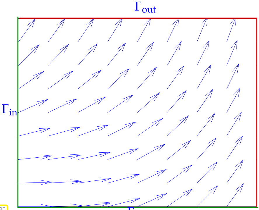
A boundary value problem depending on parameter ϵ≈ϵ0 is called singularly perturbed, if the limit problem for ϵ→ϵ0 is not compatible with the boundary conditions.
For the pure transport problem v⋅gradu=f Dirichlet boundary conditions can be imposed only on the inflow boundary part
Γin:={x∈∂Ω:v(x)⋅n(x)<0}.(10.2.1.11)
but not on its complement in ∂Ω, the outflow boundary part
Γout:={x∈∂Ω:v(x)⋅n(x)>0}.(10.2.1.12)
ϵ>0 : Dirichlet b.c. can be imposed everywhere on ∂Ω
ϵ=0 : Dirichlet b.c. can be imposed only on Γin
=> singular perturbation
On a closed streamline we cannot find a point x0∈Γin, which renders the solution formula (10.2.1.8) meaningless.
m(p) (Vertex Mass): This is the weight associated with node p, representing the area of the node patch surrounding it. It is calculated as one-third of the sum of the areas of all triangles K sharing vertex p:
m(p)=31K∈Up∑∣K∣
wh(p): The value of the test function at the node (which is 1 if wh is the basis function bp and 0 otherwise).
p.w. linear functions: grad uh is constant on each triangle but discontinuous across edges and at nodes
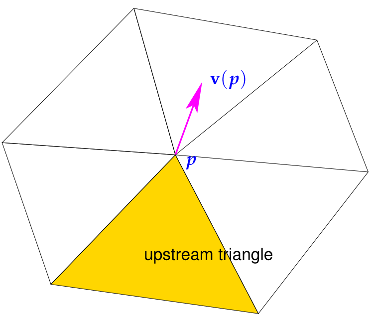
=> idea: use values from upstream triangle Ku
Ku(p):={K∈M:p∈K and ∃s>0 such that p−sv(p)∈K}
The gradient value used in the quadrature is then defined by the limit:
v(p)⋅grad uh(p):=δ→0limv(p)⋅grad uh(p−δv(p))
using “tent function” basis {bi}i=1N, entries of the convective part of the Galerkin matrix B are given by:
δK:={ϵ−1hK2hK, if 2ϵ∥v∥K,∞hK≤1,←diffusion dominated, if 2ϵ∥v∥K,∞hK>1.←convection dominated
pros: sharp jump -> no smoothing (compared to upwind quadrature)
pros: faster convergence than upwind quadrature (upwind quadrature sacrifices cvg.)
cons: (“small”) overshoots
cons: violation of max principle
"Meta theorem" :
No ϵ-robust linear method that respects the maximum principle strictly can be more than 1st-order convergent in L2!
Video 10.3.1 Method of Lines (13 min)
Method of Lines (MOL) for transient convection-diffusion problems: “half-way” discretization strategy that converts a time-dependent partial differential equation (PDE) into a system of ordinary differential equations (ODEs) by first discretizing only the spatial variables:
transient convection-diffusion equation with Dirichlet boundary conditions:
Spatial Discretization:t is treated as parameter, spatial domain is discretized (e.g., using finite elements on a fixed mesh) => system of ODEs for the time-dependent basis expansion coefficients
Mdtdμ(t)+ϵAμ(t)+B(t)μ(t)=φ(t)(10.3.1.2)
μ(t): The time-dependent vector of basis expansion coefficients representing uh(x,t).
M : mass matrix
A : FE Galerkin matrix for −Δ
B(t) : transport matrix (discretization of the convective term v⋅grad u)
φ(t) : load vector (depending on f and g -> time-independet)
Temporal Discretization: solve ODE system using numerical integrator (timestepping method) to obtain a fully discrete solution.
robustness:
spatial discretization: use ϵ-robust discretization for convective term (e.g. upwind schema)
timestepping stability: use e.g. implicit euler/SDIRK-2
12. Finite Elements for the Stokes Equations
Video 12.1 Modeling the Flow of a Viscous Fluid (30 min)
(substantial modelling component in this chapter)
thermodynamic perspective:
divv=0inΩ (incompressible)
assumptions:
small Reynolds number -> slow flows / small Ω / sticky fluid
energy dissipation mainly/only occurs in eddies -> curl
dissipation: kinetic energy -> heat
boundary conditions:
no-slip: v=0 on ∂Ω
with these assumptions, we get the space:
V:={v:Ω↦Rd continuous, divv=0,v∣∂Ω=0}.(12.1.0.6)
balance between 2nd law of T.D. (entropy maximized) and 1st law of T.D. (conservation of energy):
v∗=argmaxdissipated energy∫Ωμ∥curlv(x)∥2dx=energy injected through forces∫Ωf⋅vdx{∫Ωμ∥curlv(x)∥2dx:v∈V,v satisfies (12.1.0.12)}(12.1.0.12)(12.1.0.13)
Video 12.2.2 The Stokes Equations: Saddle Point Problem Formulation (55 min)
[AI] We want to solve a constrained minimization problem. We introduce a state space U and a multiplier space Q. For a convex differentiable functional J(v) subject to a linear constraint Bv=0, we define the Lagrangian functional L(v,p):=J(v)+(p,Bv)Q, where p∈Q is the Lagrange multiplier. The solution is found by solving the min-max problem v∗=argminv∈Usupp∈QL(v,p).
Lemma 12.2.2.4. Necessary conditions for existence of solution of saddle point problems
Any solution v∗ of (12.2.2.3) will be the first component of a zero (v∗,p∗) of the derivative (“gradient”) of the Lagrangian functional L: =DL(v∗,p∗)=0
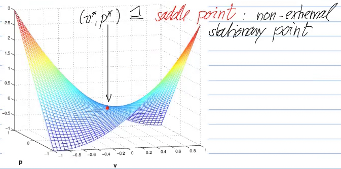
=^ solutions of min-max problems correspond to saddle points:
[AI] To find the saddle point, we evaluate the partial derivatives of L:
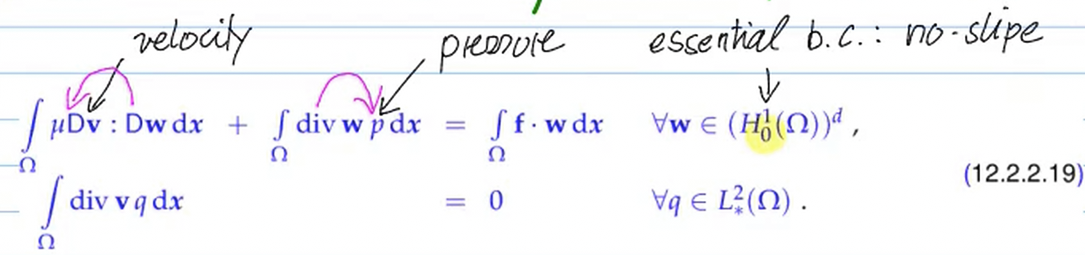
Setting the derivatives to zero yields a system of variational equations. If J(v) is quadratic, we replace DJ(v)(w) with a bilinear form a(v,w) and a linear form ℓ(w).
…we get to the variational saddle point problem (SPP)
[AI] Ensuring uniqueness of pressure: By Gauss’ theorem, ∫Ωdivvdx=∫∂Ωv⋅ndS=0 since v=0 on ∂Ω. We infer that the pressure solution p is only unique up to a constant (adding any constant c to p still retains a valid solution). To restore uniqueness, we impose a vanishing average condition on the pressure. We replace L2(Ω) with the constrained space L∗2(Ω):={q∈L2(Ω):∫Ωqdx=0}.
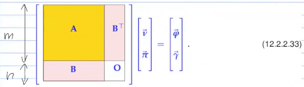
LBB2⟹N(B⊤)=0 (trivial kernel) ⟹B has full rank ⟹n≤m⟹R(B)=Rn⟹A\textbarN(B) is regular
LBB1⟹A is symmetric positive definite (elliptic) on the null space of B⟹ the saddle point system matrix is invertible, giving a unique solution for μ and π⟹∃ unique solution
example: by rising velocity field space P1→P2, checkerboard modes instability (see previous video) is cured
Definition 12.3.2.7. Stable finite element pair
A pair of finite element spaces Uh⊂H01(Ω), Qh⊂L∗2(Ω) is a stable finite element pair, if the solution (vh,ph) of the discrete saddle point problem (12.3.0.4) satisfies
where the constant C>0 may depend only on Ω, the coefficient μ, and the shape regularity measure (→ Def. 3.3.2.20) of M.
C must be independent of hM!
velocity component: unconditional stability
pressure component:
Theorem 12.3.2.15. inf-sup condition
The finite element spaces Uh⊂H01(Ω), Qh⊂L∗2(Ω) provide a stable finite element pair (→ Def. 12.3.2.7) for the Stokes problem (12.2.2.19)/(12.3.0.2) if there is a constant β>0 depending only on Ω and the shape regularity measure (→ Def. 3.3.2.20) of M such that
using residual equation + assumption + △-inequality:
discretizat. error∥u−uh∥≤independent of u(1+CsCc)best approx. errorvh∈Hhinf∥u−vh∥
-> u is quasi-optimal (optimal (see Cea’s lemma) + some constant)
Quasi-optimality: C>0 independent of data, discretization parameters
Discrete stability ⟹ quasi-optimality
If a discrete linear variational problem is stable according to Ass. 12.3.3.5, then Galerkin solutions are quasi-optimal.
which leads to:
Theorem 12.3.3.13. Convergence of stable FE for Stokes problem
If Uh,Qh is =a stable finite element pair= (→ Def. 12.3.2.7) for the Stokes variational saddle point problem (12.2.2.19), then the corresponding finite element Galerkin solution (vh,ph) satisfies
∥v−vh∥H1(Ω)+∥p−ph∥L2(Ω)≤Csum of both best approximation errors(wh∈Uhinf∥v−wh∥H1(Ω)+qh∈Qhinf∥p−qh∥L2(Ω)),
with a constant C>0 that depends only on Ω,μ, and the shape regularity of the finite element mesh.
Note: norm of velocity error also depends best-approx. error of pressure space
slower convergence error matters more!
but we don’t want a poor pressure space to affect the convergence of velocity solution:
Definition 12.3.3.16. Pressure-robust Galerkin discretization of the Stokes problem
A pair of finite element spaces Uh⊂(H01(Ω))d, Qh⊂L2(Ω) for the Galerkin discretization of the Stokes variational saddle point problem (12.2.2.19) is called pressure-robust, if the velocity component vh of the Galerkin solution satisfies
∥v−vh∥H1(Ω)≤Cwh∈Uhinf∥v−wh∥H1(Ω)
with C>0 independent of the driving force field f.
Lemma 12.3.3.17. Criterion for pressure robustness
A pair of finite element spaces Uh⊂(H01(Ω))d,Qh⊂L2(Ω) for the Galerkin discretization of the Stokes variational saddle point problem (12.2.2.19) is pressure-robust in the sense of Def. 12.3.3.16, if
and since this is a version of Galerkin orthogonality, (similar to proof for Cea’s lemma)
∥v−vh∥a≤wh∈Mh(div0)inf∥v−wh∥a
-> optimality, if approximating function in discrite space of functions with vanishing div
-> however, no practical spaces have been found that satisfy this criterion -> currently useless
Video 12.3.4 The Taylor-Hood Finite Element Method (15 min)
stable FE are balanced, if convergence (^12-3-3-13) has same order for smooth v,p
requirements for Stokes FEM:
Intermediate
The pair (Uh,Qh) of finite element spaces must be stable (→ Def. 12.3.2.7)
The velocity finite element space Uh should provide the same rate of algebraic convergence of the H1(Ω)-best approximation error w.r.t. hM→0 as the pressure space Qh in L2(Ω).
The velocity finite element space Uh should guarantee 1 and 2 with as few degrees of freedom as possible.
-> 2. and 3. concern efficiency. A stable way to satisfy the requirements is the Taylor-Hood (PS-P1) finite element method for Stokes problem:
a triangular/tetrahedral or rectangular/hexahedral mesh M of Ω, which may even be hybrid, see Section 2.5.1,
the velocity space: Uh:=(S2,00(M))2⊂(H01(Ω))d, and
the pressure space: Qh:=S10(M), which means a continuous pressure approximation.
Uh and Qh are a stable pair!
algebraic convergence, order 2 for
velocity, H1-norm
pressure, L2-norm
Video 12.3.5 The Non-Conforming Crouzeix-Raviart FEM (40 min)
non-conforming: Mh⊂(H01(Ω))d
Definition 12.3.5.2. 2D scalar Crouzeix-Raviart finite element space
The Crouzeix-Raviart finite element space on a triangular mesh M is
CR(M):={v∈L2(Ω):v∣K∈P1(K)∀K∈M,
v continuous at midpoints of interior edges of M}.
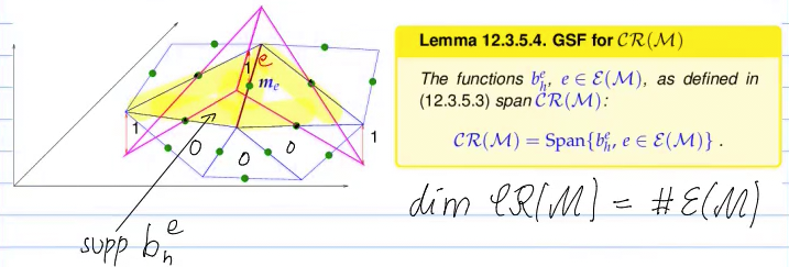
global shape functions:
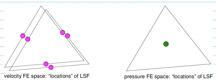
local shape functions (LSF) bK1,bK2,bK3 associated with edges of triangle K∈M:
CR-P0 FEM for Stokes:
Definition 13.1.4.38. Exterior derivative for C1 differential forms
The exterior derivative of a continuously differentiable differential form ω∈C1Λℓ(Ω) of order ℓ∈{0,…,d−1} on a domain Ω⊂Rd is the continuous differential ℓ+1-form dℓω defined asa
aIn this formula Dω:Ω→L(Rd,Λℓ(Rd)) is the (Fréchet) derivative of ω, which maps into the space of linear mappings Rd→Λℓ(Rd).
Theorem 13.1.4.57. Generalized Stokes theorem
For every domain Ω⊂Rd and ℓ∈{0,…,d−1} holds true
∫Γdℓω=∫∂Γω∀ω∈C1Λℓ(Σ),∀Γ∈Sℓ+1(Ω).(13.1.4.58)
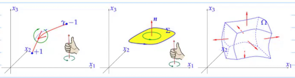
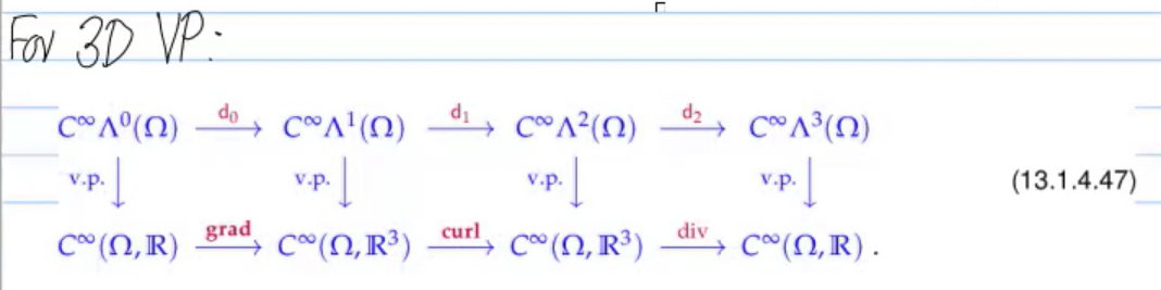
3D Vector Proxy Identifications:
d0↔grad (0-form → 1-form).
d1↔curl (1-form → 2-form).
d2↔div (2-form → 3-form).
Theorem 13.1.4.64. d∘d=0
For every domain Ω⊂Rd and ℓ∈{0,…,d−2} holds true
dℓ+1∘dℓ=0 on C2Λℓ(Ω)⇔R(dℓ)⊂N(dℓ+1),(13.1.4.65)
that is, the image of dℓ lies in the kernel of dℓ+1.
curl∘grad=0div∘curl=0
Theorem 13.1.4.81. Existence of potentials
Let Ω⊂Rd be a domain and 1≤ℓ≤d. Topological assumption: If every oriented, compact and closed⋆ℓ-dimensional sub-manifold ∈Sℓ(Ω) is the boundary of an ℓ+1-dimensional sub-manifold ∈Sℓ+1(Ω), then
Theorem 13.1.4.117. Pullback and exterior product/wedge product
Let Ω,Ω⊂Rd be two domains connected by a C1-mapping Φ:Ω→Ω. Then the pullback Φ∗ of differential forms commutes with the exterior product of differential forms:
Video 13.1.5 Sobolev Spaces of Differential Forms (18 min)
Definition 13.1.5.1. Space of square-integrable differential forms
Let u=[u1…um]⊤=:Ω→R(ℓd) by any “component representation” of a differential ℓ-form ω∈Λℓ(Ω),ℓ∈{0,…,d}.
Then we define the Hilbert space of square-integrable differential ℓ-forms
L2Λℓ(Ω):={ω∈Λℓ(Ω):ui∈L2(Ω)}.
Definition 13.1.5.2. Sobolev space of differentiable differential forms
which becomes a Hilbert space with the basis-dependent norm
∥ω∥HΛℓ(d,Ω)2:=∥ω∥L2Λℓ(Ω)2+∥dℓω∥L2Λℓ+1(Ω)2.
3. Vector Proxy Identifications (in 3D)
Form Degree
Sobolev Space
Vector Analytic Proxy
Property
0-form
HΛ0(d,Ω)
H1(Ω)
ω,grad(ω)∈L2
1-form
HΛ1(d,Ω)
H(curl,Ω)
u,curl(u)∈L2
2-form
HΛ2(d,Ω)
H(div,Ω)
u,div(u)∈L2
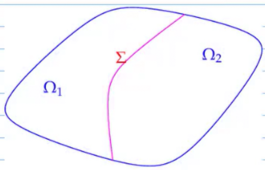
Theorem 13.1.5.10. Transmission condition for HΛℓ(d,Ω)
Let ω1∈C1Λℓ(Ω1) and ω2∈C1Λℓ(Ω2),ℓ∈{0,…,d−1}, be two continuously differentiable ℓ-forms that are continuous up to boundary of Ωi and set
ω:={ω1ω2in Ω1,in Ω2.
Then
ω∈HΛℓ(d,Ω)⇔space of tangent vectorsω1(x)(t1,…,tℓ)=ω2(x)(t1,…,tℓ)∀ti∈Tx(Σ),x∈Σ:
ω∈HΛℓ(d,Ω), if and only if the restrictions of ω1 and ω2 to Σ coincide as differential ℓ-forms on Σ.
Practical 3D Continuity:
0-forms: Global continuity.
1-forms: Tangential continuity (u1×n=u2×n).
2-forms: Normal continuity (u1⋅n=u2⋅n).
For d>1, integration over sub-manifolds is not a bounded linear functional on these Sobolev spaces (similar to how point evaluation is not bounded in H1)
Tldr: Sobolev Spaces of Differential Forms
L2-Space
coefficient functions ui∈L2(Ω)
intrinsic space (basis-independent), norm basis-dependent
Sobolev Space of “Finite Energy” Fields
HΛℓ(d,Ω):={ω∈L2Λℓ(Ω):dℓω∈L2Λℓ+1(Ω)}
Norm:∥ω∥HΛℓ2:=∥ω∥L22+∥dℓω∥L22.
The exterior derivative dℓ is a bounded linear operator mapping HΛℓ→HΛℓ+1.
Zero Boundary Conditions (H0Λℓ)
forms with vanishing tangential trace on ∂Ω
example: e×n=0 (PEC boundary conditions for the electric field, 13.1.3.43)
13.2 Discrete Differential Forms
13.2.1 Cochain Calculus (67 min)
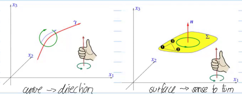
Introduce discrete integral ℓ-forms as mappings from a finite (and suitable: meaningful ∂) subset of Sℓ(Ω) into R.
reminder: Integral form: assigns value -> oriented surface
Cochain (“discrete integral form”) Assigns values to specific ℓ-facets of a mesh
ℓ-Cochain (ω): A mapping from the set of ℓ-facets Fℓ(M) of a mesh to R.
in 3D:
Cochain
assignes values to…
0-cochain
nodes
1-cochain
edges
2-cochain
faces
3-cochain
cells
Because there are a finite number of facets (Nℓ), an ℓ-cochain ω can be identified simply as a vector in RNℓ.
Definition 13.2.1.1. Generalized oriented meshes
A generalized oriented meshM of a domain Ω⊂Rd is a collection of sets of ℓ-facets,
M:=(Fℓ(M))ℓ=0d(13.2.1.1)
such that
Fℓ(M)⊂Sℓ(Ω): every ℓ-facet f∈Fℓ(M) is an oriented (*), relatively open, bounded, ℓ-dimensional, non-degenerateaCpw1-surface ⊂Rd,
for every F∈Fℓ(M),0<ℓ≤d, its boundary ∂F is the union of the closures of finitely many ℓ−1-facets:
∀F∈Fℓ(M):∃{f1,…,fm}⊂Fℓ−1(M) such that ∂F=f1∪⋯∪fm
the intersection of the closures of any two ℓ-facets is an ℓ−1-facet,
∀ℓ∈{1,…,d},∀f,f′∈Fℓ(M):f∩f′∈Fℓ−1(M)
for every f∈Fℓ(M),0≤ℓ<d, there is a F∈Fℓ+1(M) such that f⊂∂F.
aAn ℓ-dimensional sub-manifold ⊂Rd is called non-degenerate, if it has non-zero ℓ-dimensional volume.
For cochain to define values consistently, the mesh must be oriented. Each facet has an intrinsic orientation (e.g., the direction of an edge). When we look at the boundary of a face, the face’s orientation induces a direction on its edges.
Definition 13.2.1.13. Relative orientation of mesh facets
Given F∈Fℓ(M),0<ℓ≤d, and f∈Fℓ−1(M), we define their relative orientation as
or(f,F):=⎩⎨⎧1−10, if f⊂F and the orientations of f and ∂F agree,, if f⊂F and the orientations of f and ∂F are opposite,, if f⊂∂F.
example:
Definition 13.2.1.16. Exterior derivative for cochains
Given a generalized oriented mesh M of Ω⊂Rd and ℓ∈{0,…,d−1}, the exterior derivativelinear operatordℓ:Cℓ(M)→Cℓ+1(M) is defined by
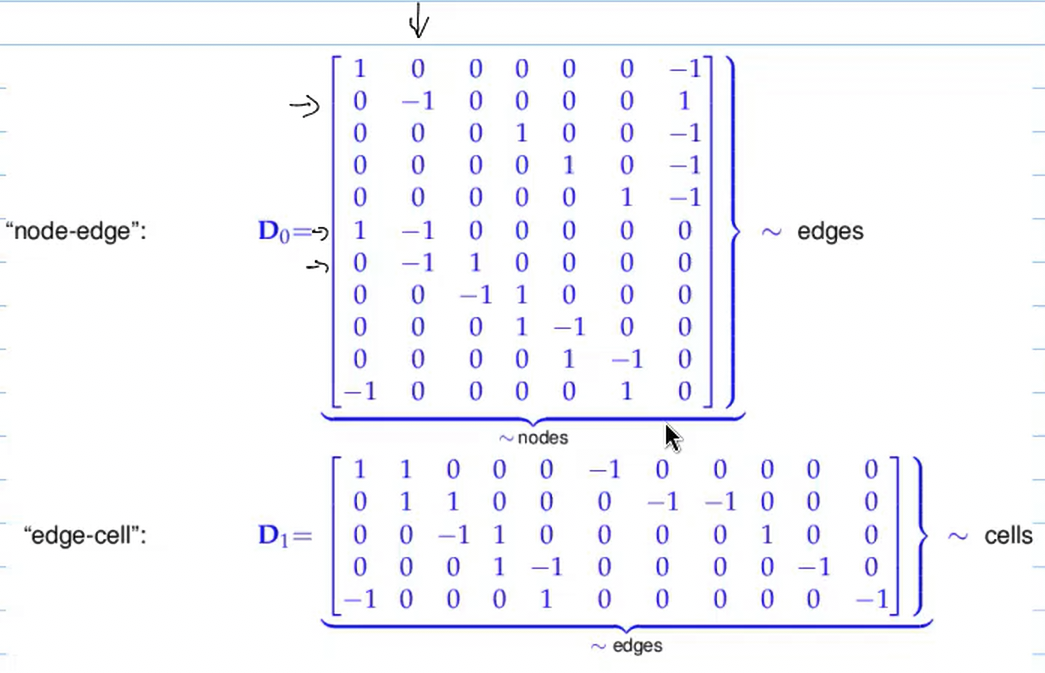
matrix representation of the discrete exterior derivative, (Dℓ)i,j=or(fj,Fi)
Matrix
Calculus Proxy
Maps…
D0
Discrete Gradient
Nodes → Edges
D1
Discrete Curl
Edges → Faces
D2
Discrete Divergence
Faces → Cells
Theorem 13.2.1.21. d∘d=0
For any generalized mesh M of a domain Ω⊂Rd and ℓ∈{0,…,d−2} holds true
dℓ+1∘dℓ=0⟺Dℓ+1Dℓ=O⟺R(Dℓ)⊂N(Dℓ+1).
the boundary of a boundary is empty
Theorem 13.1.4.81. Existence of potentials
Let Ω⊂Rd be a domain and 1≤ℓ≤d. If
(topological assumption:) every oriented, compact and closed ℓ-dimensional sub-manifold of ∈Sℓ(Ω) is the boundary of an ℓ+1-dimensional sub-manifold ∈Sℓ+1(Ω)
as a finite-element subspace of the Sobolev space HΛℓ(d,Ω) of (differential) ℓ-forms on Ω.
Convergence
reminder:if a finite-element space Vh locally contains all polynomials of degree $p$, then, for “sufficiently smooth” u, and on uniformly shape regular meshes with meshwidth hM,
vh∈Vhinf∥u−vh∥L2(Ω)=O(hMp+1)forhM→0,
here p=0, and thus algebraic cvg. of order 1
Theorem 13.2.2.59. L2-norm best approximation estimates for Wℓ(M)
If ω∈H1Λℓ(Ω) then
vh∈Wℓ(M)inf∥ω−vh∥L2Λℓ(Ω)≤CℓhM∥ω∥H1Λℓ(Ω),
with a constant Cℓ>0 that depends only on ℓ and the shape regularity measure (Def. 3.3.2.20) of M.
13.3 Whitney FEM for Computational Electromagnetism
13.3.1 Energies and Linear Material Laws (35 min)
Maxwells equations are underdetermined -> need “closure equations”
We have two 1-forms (e,h) and two 2-forms (d,b), plus the current j.
Material Laws provide the required link: they map 1-forms to 2-forms.
Field energy functionals
Electric Energy:Eel(e)=21mϵ(e,e).
Magnetic Energy:Emag(h)=21mμ(h,h).
Assumption 13.3.1.4. Linear materials
Both electric and magnetic field energies are homogeneous quadratic functionals, that is, there are bilinear forms mϵ:L2Λ1(Ω)×L2Λ1(Ω)→R and mμ:L2Λ1(Ω)×L2Λ1(Ω)→R such that
inserting this, we get:
Combining the expressions from image_1e0f33.png and image_1e0f17.png for the electromagnetic energy balance, the relationship is given by:
EM energy balancedtdE⋆(t)=−∫Ωe(t)∧j(t)+Poynting vector∫∂Ωh(t)∧e(t)=power delivered by j+power flux through ∂Ω=^ Poynting’s theorem
13.3.2.1 Electromagnetic Wave Equations (45 min)
IBVP for EM fields:
we have Maxwell’s equations, Material Laws (weak form) and b.c.
mϵ(dtde(t),e(t))+mμ(dtdh(t),h(t))⟹dtdEtot(t)=−∫Ωj(t)∧e(t).=power injected by src. current−∫Ωj(t)∧e(t)(13.3.2.14)
compared to Poynting’s theorem, power flux through ∂Ω is missing because of the b.c. -> energy change is only caused by work of source current j
use material law, differentiate in time, test with exterior derivative, 2nd term vanish (both for 1st and 2nd formula), (integration by parts), extract PDE:
todo missed some derivations that seem interesting
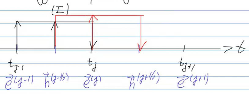
structure defines discrete Hamiltonian system -> reason why semi-descrete system (and Carank-Nicolson discretization, see later) conserve discrete Etot
some other notes:
Recall:
∫Ωb(t)∧d0v′∫Ωdtdd(t)∧d0v′=dtdd2b(t)=0∫Ωb0∧d0v′∀v′∈HΛ0(d,Ω)and all times t,=continuity equ.−∫Ωj(t)∧d0v′∀v′∈H0Λ0(d,Ω)and for all times t.(13.3.2.21)(13.3.2.27)
Observe:
d0W0Λ0(M)⊂W0Λ1(M)
d0WΛ0(M)⊂P0Λ1(M)
stage 2: timestepping -> see chapter 9.3.4 (which was not part of the course)
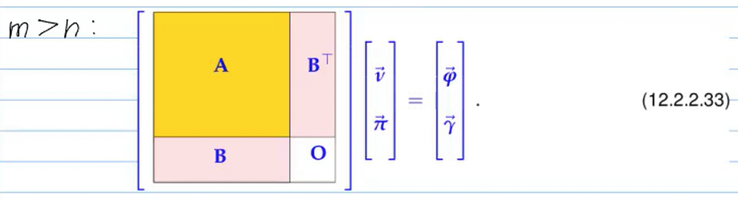
mμ∗(d1ah,d1ah′)+m(ah′,d0ph)m(ah,d0ph′)+λ=0λ∫Ωph(x)′dxorthogonality to (discrete) kernel"orthogonality to const."∫Ωph(x)dx=∫Ωj∧ah′,=0,=0.∀a′∈W1(M)∀ph′∈W0(M)∩H⋆∧0(d,Ω)(13.3.3.33)
then the discrete variational saddle point problem (12.2.2.49) possesses a unique solution (vh,ph)∈Uh×Qh, which satisfies the Galerkin discretization error estimate
We’re converting image into markdown + latex formulas. For normal text, normal markdown. For boxes, use callouts. The format of callouts is the following:
> [!name] <title>> > content
Note that there is no empty line between the callout header and the content!
orange boxes: convert to !intermediate
lemmas, theorems (yellow): convert to !lemma, !theorem
definitions (red): convert to !definition
For inline latex, the format is the following: <content>
For one-line latex, the format is the following:
<content>
note the newlines in between $$ and the content
for latex blocks in callouts, please do not write newlines: if possible, the whole latex block should be on one line
For multiline latex, the format is the following:
<content>
Highlighted text can be highlighted in markdown, too: highlight. This is not standard commonmark, but if you see highlighted text in the image, highlight it when converting, too. Same for bold: if a text is emphasised, make it bold.
Note that highlighting can only be used for markdown, not for latex
If something cannot be converted to pure markdown, warn me instead of attempting to use non-standard syntax.
For this task, you may omit any custom formats specified earlier.
Your answer should consist solely of the markdown (and the warning if something cannot be converted). No follow-up suggestions, questions, clarifications.
for colors in latex, use \textcolor{color}{content} instead of \color{color}{content}
whenever possible (i.e. for latex blocks (not inline)), use \tag{...} to write the number

 -> but need formula for potential energy
 Note:

 Recall from LA:

Thus, for of solution, the problem must fulfill:
 choose
 in contrast to -Space, here the boundary conditions are not dropped; the reason for this are the norms:
 Sobolev space without boundary conditions:
 the can be bounded by the size of the domain and the energy norm:
 Poincare-friedrich?


 => 2-pt BVP (a Dirichlet problem) in strong form (vs. “weak form” = LVP)
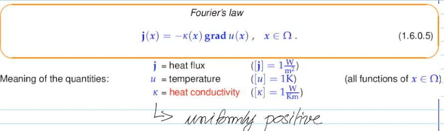 by combining those two using Gauss theorem, we get:
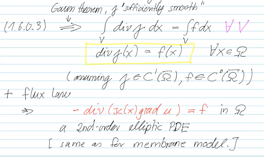 => we reach at the same PDE as for the membrane model
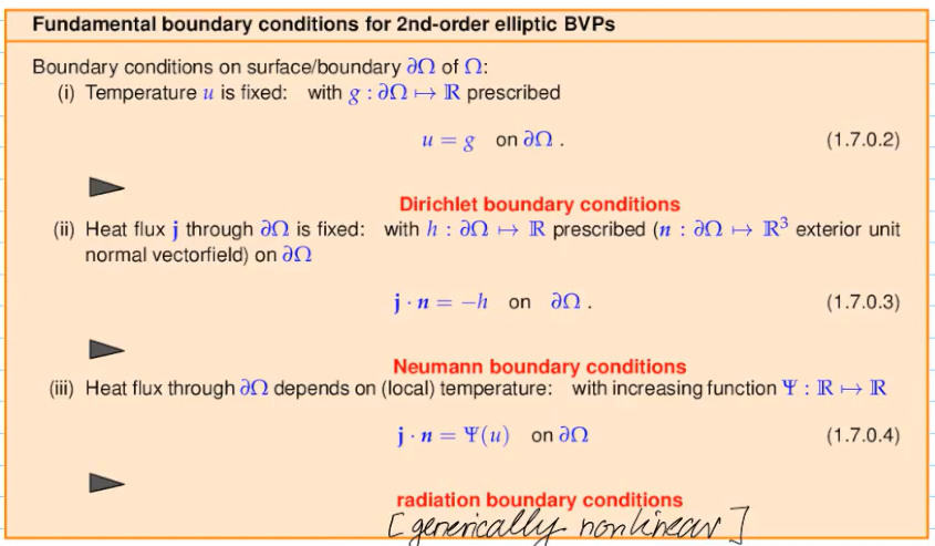 example of a mixed BVP:
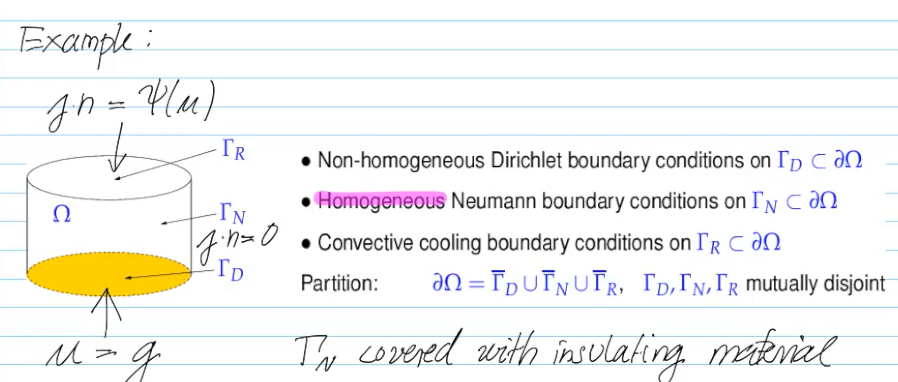
 for Dirichlet BVP:
 for Radiation BVP:
 for Neumann BVP:







 there are two approaches to creating the Galerkin-matrix:
 Problems:
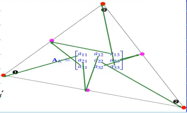
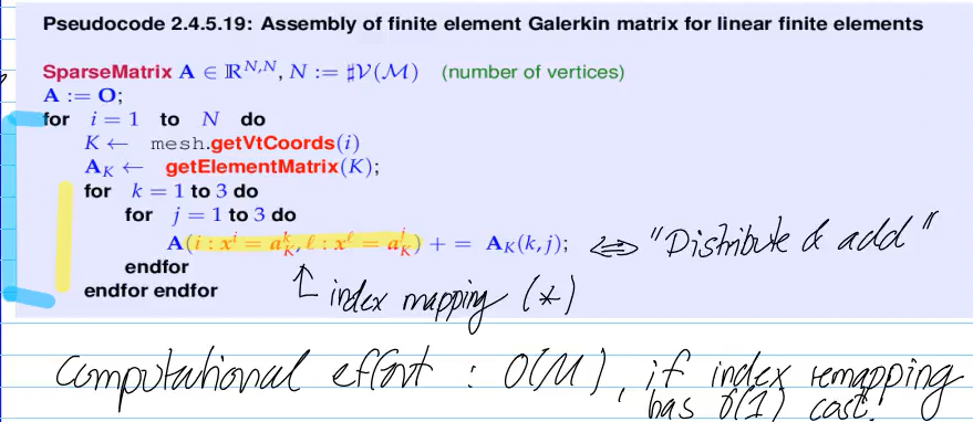
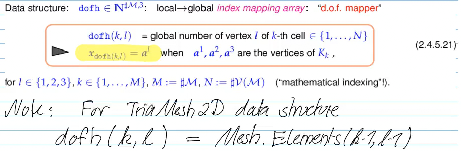 dof: degrees of freedom
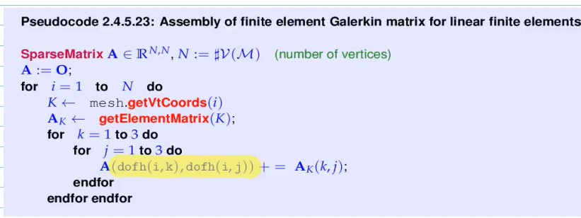
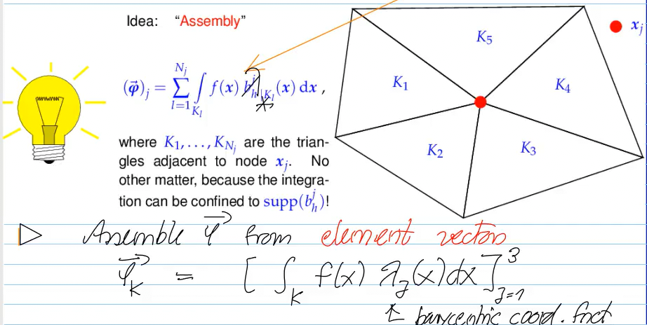 for the RHS, we can compute the integral using composite trapezoidal rule (we are working with triangles anyways):
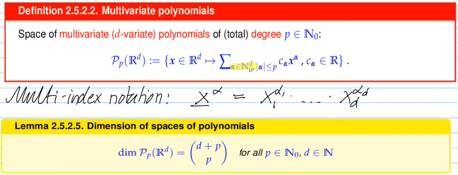 1st option: e.g.
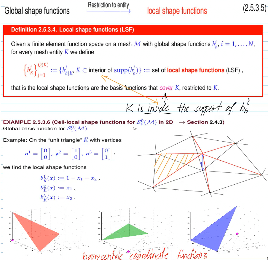
 one triangle, with Kardinal property:
 gluing triangles (interpolation nodes):
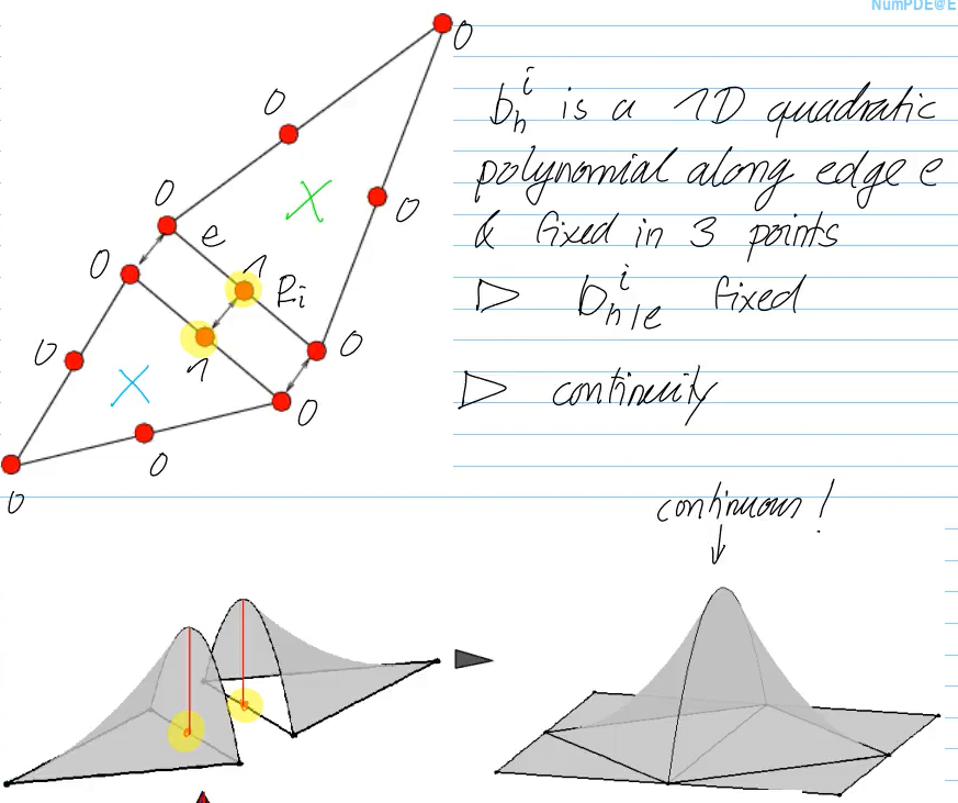 -> globally continuous piecewise function
 for hybrid mesh:
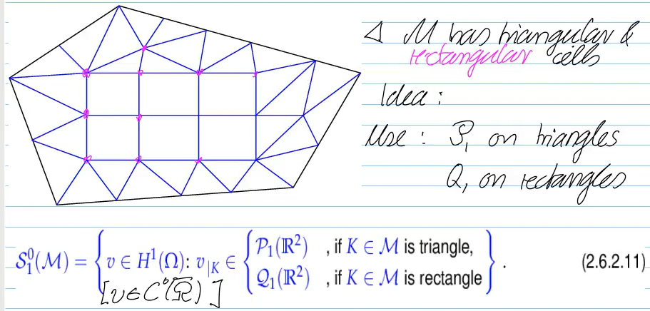 works, becuase functions are all linear when restricted to straigt edge (which we have)
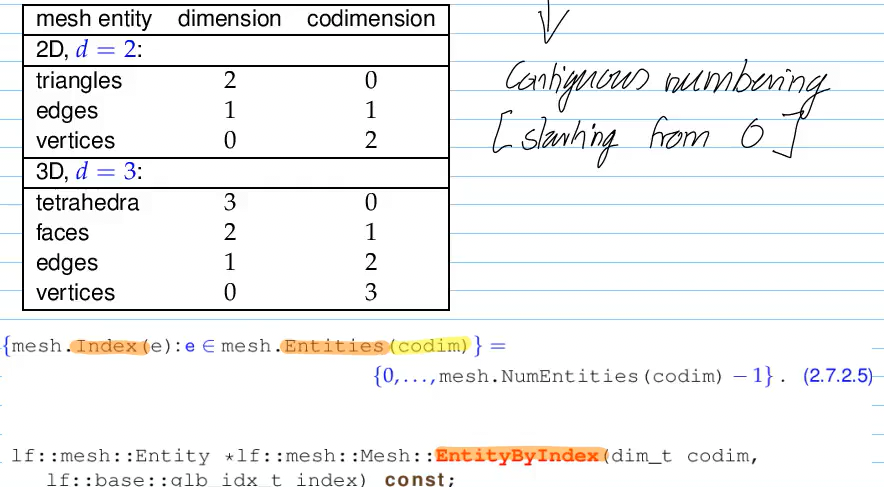
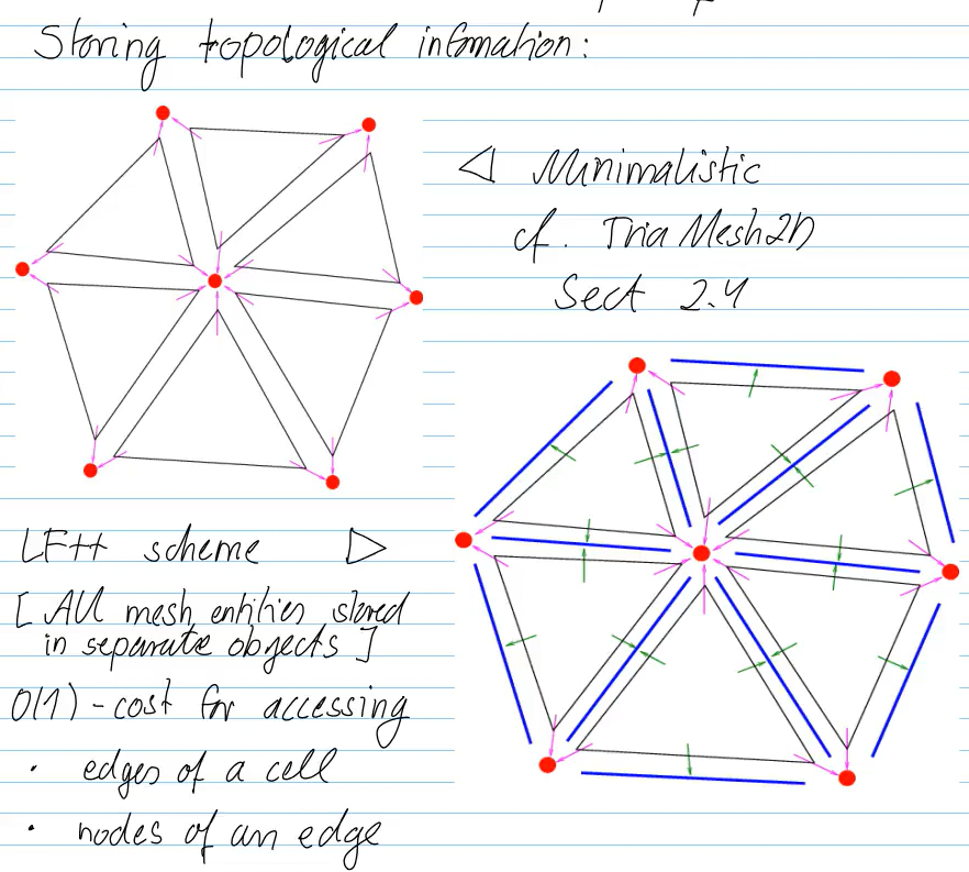 access:

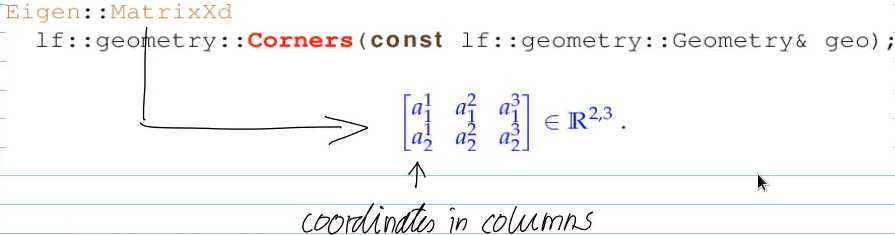
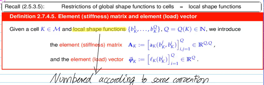
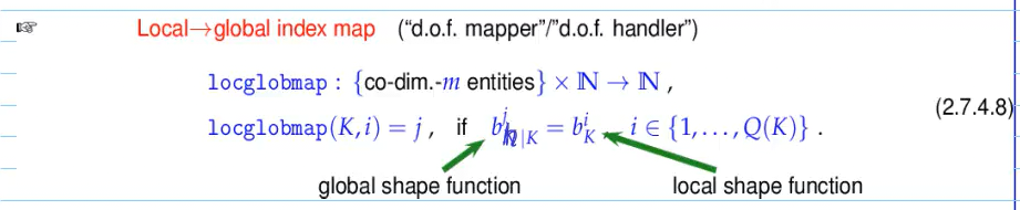
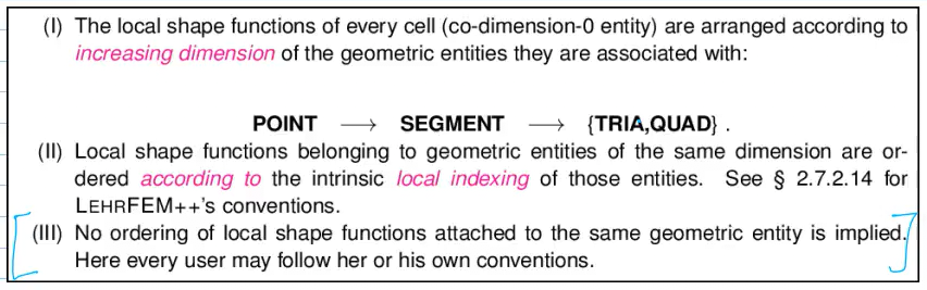
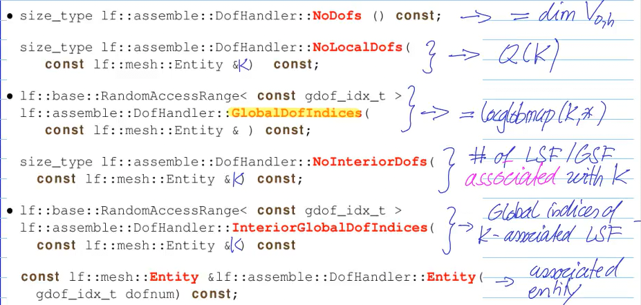
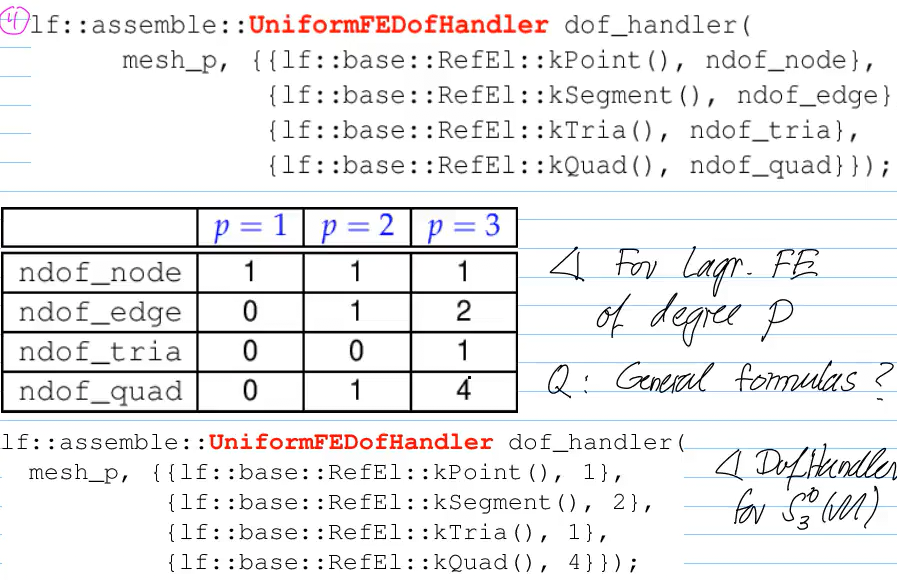
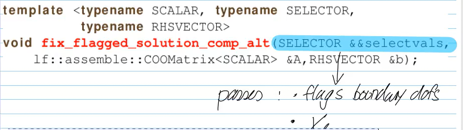
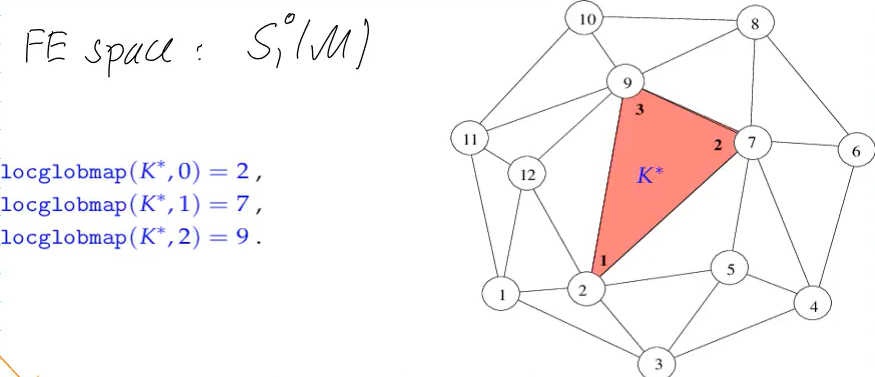 LehrFM numbering rules:
 for lagr. FE: uniform no of GSFs associated with entities of same type -> initalization can be simplified:
 distribute pattern used for assembly
 local quadrature
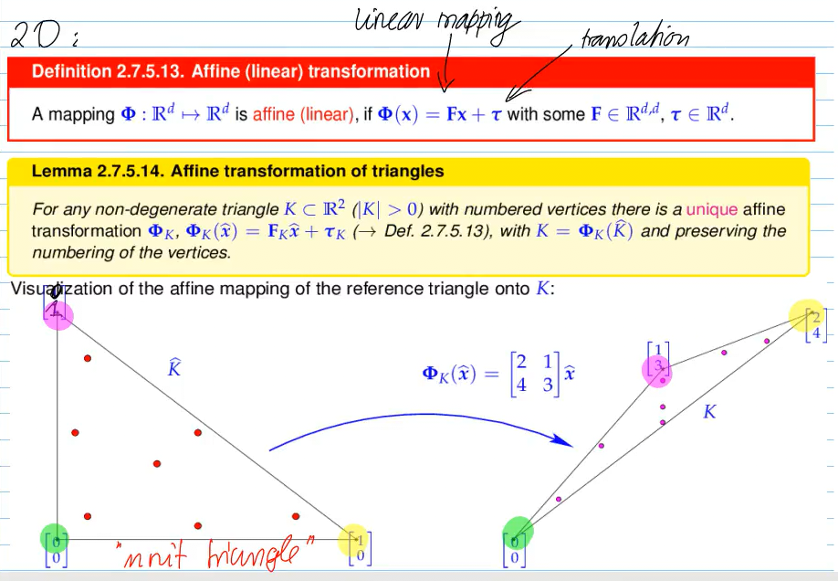 (affine mapping maps lines to lines)
 example on :
 however, if affine => , and we get:
 in LehrFEM, we can use:
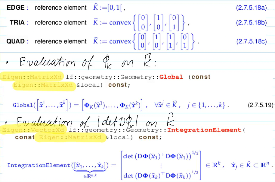
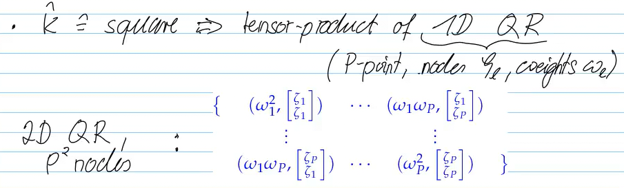 quadrature rules in LehrFEM: reference object shape + desired order

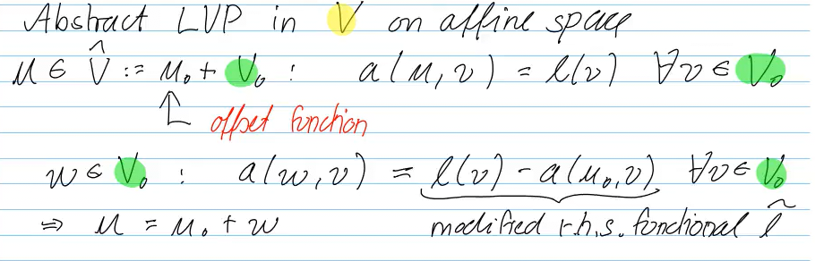
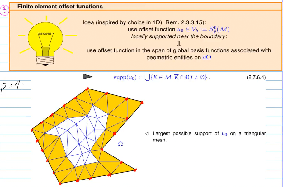
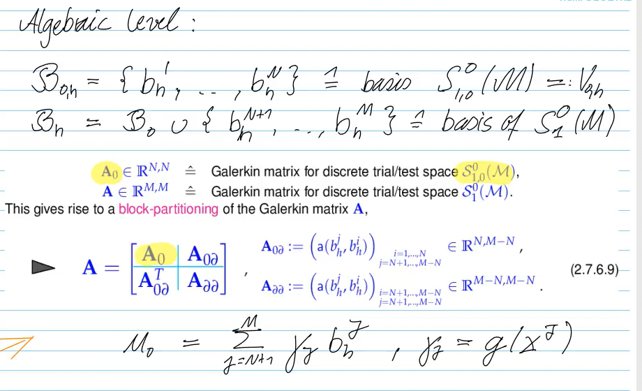
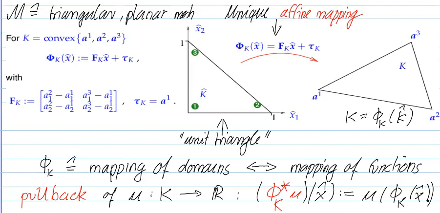 affine pullback preserves polynomials:
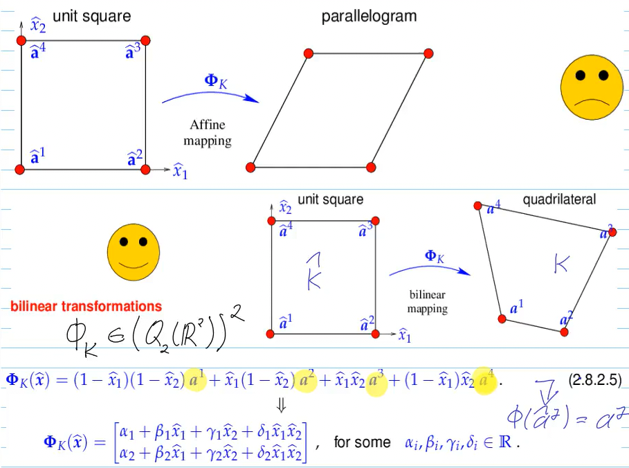
 Note that possibility of gluing needs to be checked!
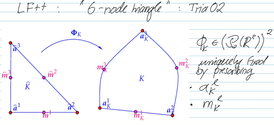
 “6-node triangle” in LehrFEM++:
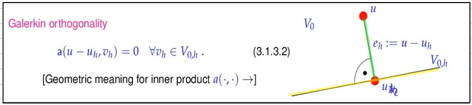 from this follows Pythagoras theorem:
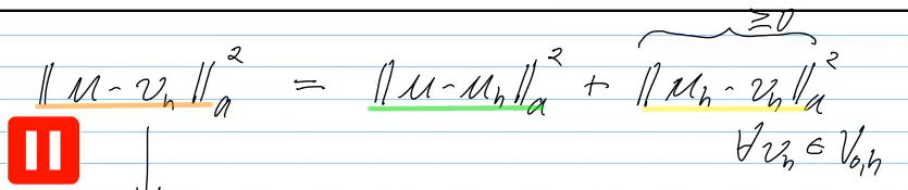
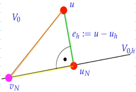 or shorter:
 using localization and fourier law, we get:
 necessarily implicit
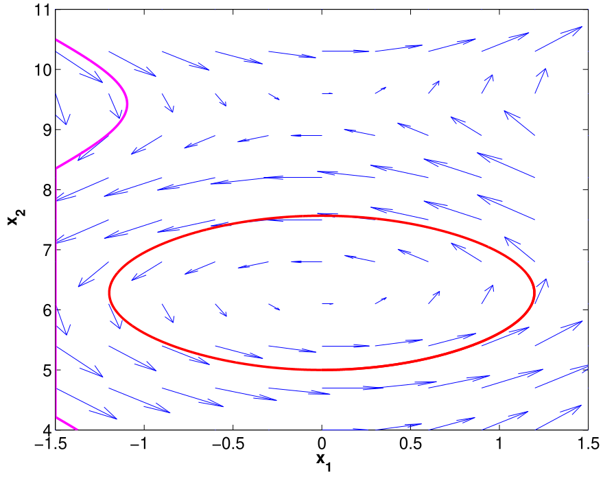
 upwind quadrature rule approximates the convective bilinear form as a weighted sum over all mesh nodes :
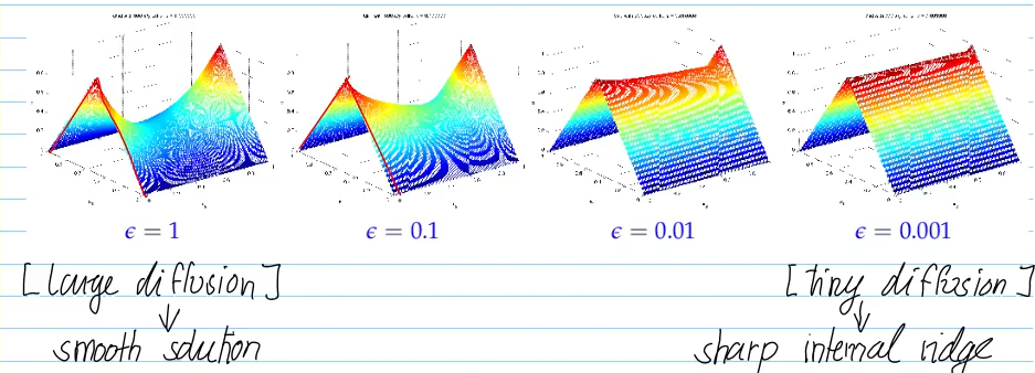 enhancing diffusion smearing of internal layers and ridges
 [AI] To find the saddle point, we evaluate the partial derivatives of :
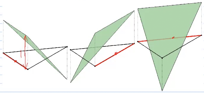 CR-P0 FEM for Stokes:
 DVP: seek such that
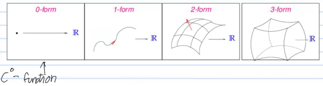 Notation: vector space of -forms