links - Theoretical Astrophysics
Info
- exercises
- if difficult topic: recap
- if “simple” topic: solving exercises together in class
Exam Theoretical Astrophysics
100% oral exam
Exercises
-> HS2026_tasks
| Serie | Lösung | master solution | Korrektur |
|---|---|---|---|
| 20260930_Astro_Ex1.pdf | 20260930_Astro_Solution1.pdf | ||
| 20261006_Astro_Ex2.pdf | 20261006_Astro_Solution2.pdf |
Vorlesung
TODO:
- chapter 1.2/1.3? - do not understand how we got to with a correction term (I think something like )
Introdution
1. Intro solar system
solar system
- Structure: The Sun contains over of the solar system’s mass. It is orbited by eight planets, numerous satellites, and small ice/rock bodies (e.g., Eris).
- Orbital Characteristics: Planets move in nearly circular, concentric orbits along the same plane (ecliptic, within ) and direction.
- Moons: All planets except Mercury and Venus have moons. Most moons and planets spin in the same direction as their primary orbits. Some satellite systems are larger than smaller planets.
the sun
- Properties: A G2-type star containing the mass and the volume of Earth. Energy is produced via hydrogen fusion in its core ().
- Internal Structure:
- Core: Extends to of the Sun’s radius; holds of the volume and about of the mass.
- Convection Zone: Outer radius where heat circulates in giant gas bubbles, visible on the surface as granules that last 5–10 minutes.
- Photosphere & Helioseismology: Surface oscillations reveal differential rotation (equator rotates faster than poles) and internal jet streams.
- Surface Activity & Magnetism:
- Sunspots: Cool regions ( lower than surrounding areas) tied to strong magnetic fields. They follow an cycle.
- Phenomena: Differential rotation winds up magnetic field lines, causing loop releases that display as sunspots, prominences/coronal loops, and solar flares across the EM spectrum.
- Solar Wind: A stream of electrons and protons escaping through coronal holes, causing auroras on Earth.
planetary categories
- Terrestrial Planets (Mercury, Venus, Earth, Mars): Small, dense, rocky worlds located in the inner solar system with relatively thin atmospheres.
- Giant Planets:
- Jupiter: Most massive planet ( mass of all other planets combined). Features a gaseous, cloud-covered surface, the Great Red Spot storm, and at least 63 moons (including the 4 main Galilean satellites).
- Saturn: A gas giant with of Jupiter’s diameter but only of its mass. Famous for thin ( thick) water-ice rings maintained by moon gravitational interactions.
2. Milky Way
multi-wavelength observations
- Visible light reveals obscuring dust, whereas Near-Infrared (NIR) exposes the thin disk structure.
- Far-Infrared (FIR) isolates dust distribution, emission maps neutral hydrogen gas (), and lines trace active star-forming regions.
Disk Structure & Kinematics
- Thin Disk: Scale height/thickness of ; contains stars, dust, and gas enabling active star formation.
- Galactic Rotation: Radial velocity measurements (e.g., via CO lines and Gaia/OGLE data) under flat rotation models () allow mapping of inner and outer disk structures.
- Solar Location & LSR: Distance to Galactic Center (): (GRAVITY 2019; IAU conventional value )
- Local Standard of Rest speed: .
- Solar peculiar motion: relative to the LSR.
Bulge, Halo, and Clusters
- Galactic Bulge: Displays an “X” shape / boxy profile driven by dynamical instabilities.
- Star Clusters:
- Open Clusters: Young ( older than ), loosely bound ( stars), concentrated in the disk plane to trace spiral arms.
- Globular Clusters: Old (up to ), densely packed (up to stars within ), distributed spherically in the stellar halo ( known).
- Stellar Halo: Extends out to ; contains metal-poor stars, globular clusters, dwarf satellite galaxies, and stellar streams formed from tidal galaxy mergers.
stellar populations
- Population I: Metal-rich stars located in the disk and spiral arms with near-circular orbits.
- Population II: Metal-poor stars in the bulge and stellar halo with eccentric orbits.
- Population III: Hypothetical, first generation of extremely metal-poor stars.
- Modern View: Components are categorized by distinct structural regions (thin disk, thick disk, bulge, stellar halo, dark matter halo) linked to specific stellar populations and metallicity profiles.
3. Interstellar Medium (ISM)
the gas and dust filling the space between stars
ISM composition
- Gas: Composes the vast majority of the ISM. Consists primarily of hydrogen and helium, with trace amounts (<1%) of heavier elements.
- Dust: Consists of larger, soot-like complex particle clumps.
Interstellar dust, effects
- Extinction & Reddening: Dust blocks background starlight (extinction) and preferentially absorbs shorter (blue) wavelengths, making distant objects appear redder (reddening). Reddening changes the continuum spectrum but does not shift spectral lines (unlike Doppler redshift).
- Thermal Emission: Dust grains absorb starlight, warm up, and re-emit energy continuously, peaking in the infrared (IR) spectrum.
- Infrared Piercing: Infrared light penetrates dust far better than visible light, revealing stars and structures hidden behind dark clouds.
gas oservation Gas is observed via three main spectral methods:
| Gas State | Detection Method | Visual / Physical Characteristics |
|---|---|---|
| Hot Gas Clouds | Visible emission lines | Heated and ionized by UV radiation from hot young stars (e.g., H red light from hydrogen; green light from ionized oxygen transitions). Indicates recent star formation. |
| Neutral Hydrogen | 21 cm radio lines | Allows mapping of cold gas throughout the galaxy. |
| Cold Dark Clouds | Radio spectral lines from molecules | Cold, dense regions where molecules form. |
dark clouds & interstellar molecules
- Environment: The densest regions of dust clouds are very cold (). Dust blocks UV radiation, allowing molecules to form and survive without being photoevaporated.
- Radio Detection: Rotational state transitions of molecules emit radio photons, which pass through dust unhindered.
- Key Species: While molecular hydrogen () is most abundant, it does not emit in the radio spectrum. Carbon monoxide () is the primary tracer due to its abundance and easy excitation at low temperatures. Other molecules include (formaldehyde), , , and complex organic compounds.
The Local Bubble
- UV space astronomy reveals that the ISM contains hot, low-density “bubbles” and “tunnels.”
- The interior emits UV spectral lines, while the cooler outer shell emits 21 cm neutral hydrogen radiation.
- Our Sun resides inside the Local Bubble—a region roughly 100 parsecs across containing stars, likely carved out by ancient supernova explosions.
4. Stellar Evolution
timestamp 2026-09-21
- Mass-Luminosity Trade-off: More massive stars burn hydrogen faster and die much sooner.
- Nuclear Fusion: Core hydrogen fuses into helium via the chain (low mass) or CNO cycle (high mass).
Low to Intermediate Stars () -> Evolution: Main Sequence Red Giant (RGB) Horizontal Branch Asymptotic Giant (AGB) Planetary Nebula White Dwarf
- Helium Flash: Stars below develop a degenerate helium core. Core helium ignition occurs explosively once temperatures rise enough.
- Final Remnant: Planetary nebula ejects the outer layers, leaving behind a Carbon-Oxygen White Dwarf held up by electron degeneracy pressure.
Massive Stars () -> Evolution: Main Sequence Supergiant Onion-Skin Shell Burning Core-Collapse Supernova Neutron Star / Black Hole
- Onion-Skin Burning: Successive core/shell burning stages grow shorter and hotter:
- The Iron Boundary: Fusing Iron () absorbs energy rather than releasing it.
- Core Collapse: When the iron core reaches the Chandrasekhar limit ():
- Photodisintegration breaks iron nuclei.
- Electron capture () neutralizes protons.
- Outer layers collapse onto the dense core, bounce off, and trigger a Type II Supernova.
- White Dwarf: Supported by electron degeneracy pressure ().
- Neutron Star: Supported by neutron degeneracy pressure ().
- Black Hole: TOV limit exceeded; gravity overwhelms all degeneracy pressure ().
| Star Mass (M) | Core Ignition | Final Burning | Remnant Type |
|---|---|---|---|
| None | None | Brown Dwarf | |
| Hydrogen | Hydrogen | He White Dwarf (Hypothetical) | |
| Helium (Flash) | He / C-O | C-O White Dwarf | |
| Full Chain (Fe) | Silicon Iron | Neutron Star | |
| Full Chain (Fe) | Silicon Iron | Black Hole |
5. Galactic structure
- Central bulge, bar: Central, rounder galaxy region. Ranges from a spherical “classical” bulge to a flattened “pseudo-bulge” or bar. dominates galactic dynamics within a few of the center. Surface-brightness profile well represented by a Sérsic profile
- Galactic Disk: A flattened structure extending radially from the center containing stars and gas. Its radial light distribution generally follows an exponential profile
- Stellar Halo: A surrounding structure containing stars and globular clusters. Contains relatively little mass (e.g., in the Milky Way), but acts as a tracer population where dark matter dominates
- Dark Matter Halo: A vast, surrounding halo of dark matter that dominates the total mass profile and dynamics of the galaxy at larger radial distances ().
6. Active Galactic Nuclei (AGN)
-> main point: different classes of AGNs are fundamentally the same physical system viewed from different angles/having varying jet activity
components
- Central Supermassive Black Hole (SMBH): A black hole with, , drives the system via matter accretion
- Broad-Line Region (BLR): Fast-moving gas clouds close to black hole (), emitting broad emission lines due to high-velocity orbital motion
- Narrow-Line Region (NLR): Slower-moving gas clouds located further out from the central engine -> narrower emission lines
- Dusty Torus: A doughnut-shaped ring of thick dust and gas surrounding the inner regions (accretion disk and BLR). Depending on the line of sight, this torus obscures the central engine and BLR
- Relativistic Jets: Collimated outflows launched perpendicularly to the accretion disk.
The unified model posits that different observed classes of Active Galactic Nuclei (AGN) are fundamentally the same physical system viewed from different angles or possessing varying degrees of jet activity.
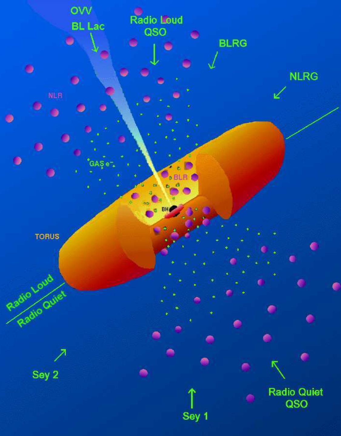
| orientation | explanation | classification |
|---|---|---|
| unobscured (face-on) view | looking down the opening of the dusty torus; BLR and NLR visible | - seyfert type 1 - QSOs |
| obscured (edge-on) view | dusty torus blocks line of sight to center; only NLR visible | - seyfert type 2 - NLRGs |
| line-of-sight alignment (Blazars) | looking directly down the axis of the relativistic jet; large variability | - OOV - BL Lac |
- BL Lac = blazars
- OVV = optically violently variable
- BLRG = broad-line radio galaxy
- NLRG = narrow-line radio galaxy
- Sey 1= Seyfert type 1 (broad emission lines visible)
- Sey 2 = Seyfert type 2 (only narrow emission lines visible)
TLDR - AGNs
All AGN’s are (could be) the same model, looked at either from the side (central black hole hidden) or from the top (torus, black hole visible). If the view is directly centered on the jet, we get Blazars (strong emissions) -> perspective determines AGN type
| Radio-strong | Radio quiet |
|---|---|
| strong jet | weak / no jet |
| radio-loud QSOs, BLRG, NLRG, Blazars | Seyfert 1&2, Radio-quiet QSOs |
7. EXTRA: EBL
Extragalactic Background Light (EBL) is the accumulated diffuse radiation emitted throughout the history of the Universe by extragalactic sources, primarily driven by star formation (nucleosynthesis) and active galactic nuclei / black holes (gravitation). Total EBL is equivalent to of the Cosmic Microwave Background (CMB)
- Absolute EBL/CIB measurements are difficult due to local foregrounds like zodiacal light and Galactic dust/cirrus
Zodiacal light
A faint, triangle-shaped glow in the night sky that is caused by sunlight reflecting off interplanetary dust
| Spectrum Component / Waveband | Primary Integrated Brightness (nW⋅m−2⋅sr−1) PDF | Key Sources & Physical Drivers PDF |
|---|---|---|
| Cosmic Microwave Background (CMB) | Thermal blackbody radiation (). | |
| Cosmic Infrared Background (CIB) | Dust emission, star formation, and energy production history post-recombination. Note that . | |
| Cosmic Optical Background (COB) | Direct starlight and optical emission from distant galaxies. | |
| X-Ray Background (XRB) | High-energy emission from AGN, accreting black holes, and Seyfert galaxies. Peak energy is around . | |
| Gamma-Ray Background (GRB) | Diffuse high-energy emission driven largely by blazars (FSRQs and BL Lac objects). | |
| Radio Background | () | Low-frequency synchrotron and non-thermal emission from radio-loud extragalactic sources. |
1. Stars
1.1 Hydrostatic EQ
Assumption: spherical sym. in stars
- : mass enclosed
- : mass of spherical shell
if we take a combination:
- at :
- at :
=>
total grav. pot energy
total energy
- :
- : <
recap - ideal gas
- monoatomic:
- diatomic (fixed bond length): (3 translational, 2 rotational)
- total internal energy:
recap - specific heat capacity
-> when volume/pressure is fixed, how much energy is needed to increase temp
- polytrope index: for mono, for di, for radiation
=> back to the stability condition:
and (similar to virial theorem)
note: If we use monoatomic gas (), we exactly get the virial theorem
-> the gravitational system has negative specific heat capacity!
* adiabatic case
-> -> => polytropic relation
Kevin-Helmholtz time scale
Assuming + in hydrostatic equilibrium, we get
and we get the
-> short!; needs additional energy source -> fusion
radiative transfer basics
timestamp 2026-09-29
Extra material for 1.2 Radiative Transfer from Rybicki & Lightman 1.1 – 1.5
- specific intensity : bundle of rays (), surface brightness
- flux:
- pressure:
- specific energy density:
- Planck distribution for black body:
- approximations & laws:
- sources that may/may not be B.B. (not even full spectrum avail.):
- brightness temp.:
- color temp.:
timestamp 2026-09-29
- specific intensity
- flux: number of photons in a given area per unit time
- energy density (zero moment??)
- flux (first moment)
- pressure (2nd moment)
example:
adiabatic case :
1.2 Radiative energy transfer
since not moving, energy transfer has either to be conduction or radiation (though conduction is low)
scattering
\implies 0 = -c \nabla_{j} p^{ij}- \rho F_{\nu}^i (\underbrace{ K_{\nu}^\text{abs} + K_{\nu}^\text{out}-K_{\nu}^{in} }_{ K_{\nu}^\text{tot} })$$
c \nabla_{i}p^{ij} = \rho F_{\nu}^i K_{\nu}
\begin{align} K_{\nu}^\text{out} - K_{\nu}^{in} & = \int d^2 \hat{n}’ K_{\nu}^\text{out} (n\to n’) - \underbrace{ \int d^2 \hat{n}~\hat{n}\cdot \hat{n}‘~K^\text{in}(n’\to n) }{ \int d^2 \hat{n}‘\hat{n}‘\cdot \hat{n} ~K^\text{in}(n\to n’) } \ \ & = \int d^2 n’(1-n\cdot n’)K{\nu}(n\to n’)
\end{align}
> [!tldr] ?? > changing in time over given observation. $I_{v}$ has all information but is complicated function $\to$ integrate for static moment, compute second moment (pressure gradient in radiation field) depends on total flux and total opacity #### 1.3 Radiative models > #timestamp 2026-10-05 ##### additional: Hertzsprung-Russel diagram Here is a concise summary of the core concepts covered in the documents: **Hertzsprung-Russell (H-R) Diagram** A plot mapping stellar luminosity / abs. magnitude against effective temperature ($T_{eff}$) / surface temp / spectral type Key regions * **Main Sequence (MS)**: Contains about 90% of all stars, forming a diagonal band from high-temperature/high-luminosity down to low-temperature/low-luminosity (the Sun is a main sequence star). * **Red Giants (RGs)**: Cool, highly luminous stars positioned above the main sequence. * **Supergiants (SGs)**: Extremely luminous and massive stars occupying the top region across various temperatures. * **White Dwarfs (WDs)**: Hot, small, low-luminosity stars located below the main sequence. **Physical relationships & rules** * **Mass-Luminosity Relationship**: For main sequence stars, luminosity scales with mass according to $L \propto M^\alpha$ (where $\alpha \approx 2$ to $4$, averaging around $3.3$). Higher-mass main sequence stars are far more luminous and rare. * **Main Sequence Limits**: * **Lower limit**: ~0.08 $M_\odot$; objects below this threshold cannot ignite hydrogen fusion (brown dwarfs). - **Upper limit**: ~100 $M_\odot$; stars above this limit are disrupted by radiation pressure (exceed eddington limit) * **Main Sequence Lifetimes**: stars lifespan is related inversely: $t_{\text{MS}} \propto M^{-2.3}$. Massive stars burn fuel rapidly and live significantly shorter lives than low-mass stars - evolution * **Low-mass stars** (e.g., the Sun) $\rightarrow$ Red Giant $\rightarrow$ Planetary Nebula ejection $\rightarrow$ **White Dwarf**. * **High-mass stars** $\rightarrow$ Supergiant $\rightarrow$ Supernova explosion $\rightarrow$ **Neutron Star** or **Black Hole**. #### 1.4 Opacity Rosseland mean opacity\int dv~ \frac{4\pi}{dv} \frac{dB_{v}}{dT} = \frac{1}{k_{R}} \int dv~ \frac{4\pi dB_{v}}{dT}
\begin{align} k_{\text{tot}} & =k_{\text{abs}}+k_{\text{out}} - k_{\text{in}} \ k_{\text{out}} & = \frac{1}{m_{p}} \int d^2n’~ \sigma(n\to n’) \ k_{\text{in}} & = \frac{1}{m_{p}} \int d^2n’~ (\hat{n}\cdot \hat{n}’)\sigma(n\to n’) \end{align}
\implies k_\text{tot}=k_{0}\underbrace{ \left( \frac{\rho}{\rho_{0}} \right)^\alpha\left( \frac{\kappa T}{\kappa T_{0}} \right)^\beta }_{ \text{both dimensionless} }
> [!question] TODO: Why is $k_{in}$ $k_{out}$ with the factor $(\hat{n}\cdot \hat{n}')$? -> unanswered from chapter 1.2 > but what is opacity?\frac{1}{c} \frac{\partial}{\partial t} I_{\nu}\sim \hat{n}\cdot \nabla I_{\nu}\sim \kappa_{\nu}\rho I_{\nu}
so $[\kappa_{\nu}\rho] = \frac{1}{L}$ typically written in form of scattering cross-section\sigma_{\nu},\quad\quad \frac{d\sigma_{\nu}}{d\Omega}d\Omega
![[HS2026/Attachments/Untitled-2026-10-06-1024.excalidraw(2).svg|400]] (includes all kinds of interactions - week nuclear, strong, ...) -> there are many cases, each one different **ionized hydrogen gas** ($m_{p}$: proton mass)\begin{align} H1 & = e^- & p^+ \ H 2 & =e^- + p^+ \ \rho & =\frac{N\cdot m_{p}}{V}=n\cdot m_{p} \ \implies \kappa \rho & = n\sigma \iff \kappa = \frac{\sigma}{m_{p}} \end{align}
- **Thompson** (classical) scattering for charged particles - **Bound-Bound**: electronic transition - there are also atomic, molecular transitions - **Bound-free**: photo-ionization $13,6eV$, recombination - **freee-free**: Bremsstrahlung - (btw: inverse Bremsstrahlung $\hat{=}$ absorption) **Example: thompson scattering** ![[HS2026/Attachments/Untitled-2026-10-06-1024.excalidraw.svg|400]] (scene embedded in svg) - for $E\nu\ll m_{e}c^2$ elastic - for $E\nu\gg m_{e}c^2$ compton scattering:\begin{align} \lambda_{f}-\lambda_{i} & =\frac{h}{m_{e}c}(1-\cos \vartheta) \ \frac{d\sigma}{d\Omega} & \frac{\sim_{1}}{x} & x = \frac{h\nu}{m_{e}c^2}\gg1 \ & & x\ll_{1} \end{align}
\begin{align} \sigma(n\to n’) & = \frac{3}{16\pi} \sigma_{t}\left[1+(\hat{n}\cdot \hat{n}’)^2 \right] = \frac{d\sigma}{d\Omega}d\Omega\ \sigma_{t} & = \int d\Omega~ \frac{d\sigma}{d\Omega}=\frac{8\pi}{3}r_{0}^2 = 6.6\cdot 10^{-25}\text{cm}^2 \sim \frac{1}{m^2} \ m_{e}c^2 & = \frac{\epsilon^2}{r_{0}}\quad \nu_{0}\sim 2.8\cdot 10^{-13}\text{cm (?)} \end{align}
> [!important] cross section $\sigma_{t}$ is important aspect (whatever that means) > ---\begin{align} \frac{1}{c} \frac{\partial}{\partial t}I & = -\hat{n}\cdot \nabla I\quad -n_{e}\sigma \cdot I \ \frac{d}{ds} I & = -n_{e}\sigma I \ d \ln(I) & = -n_{e}\sigma ds \ I & \sim e^{-\lambda} \ \text{optical depth}\quad \lambda & =\int ds\cdot n_{e}\cdot \sigma \ d\lambda & \equiv n_{e}\sigma \cdot ds \end{align}
- if $n_{e}, \sigma$ not dependent on $s$ -> simple integration; otherwise, you get frequency (has to compute integral)\begin{align} \lambda=1 & = n_{e}\sigma \cdot s \ & = \underbrace{ \frac{S}{L} }{ \text{typical length} } \ \frac{1}{L} & \equiv n{e}\sigma = \kappa \rho & \text{mean free path} \end{align}
\begin{align} \sigma & \sim 10^{-25}\text{cm}^2 \ n_{e} & \sim 10^{-24}/\text{cm}^3\ \rho & = \frac{\mathcal{M}}{V}\sim 1 \frac{g}{\text{cm}^3} \ n_{p} & \sim 10^{24} / \text{cm}^3 \ \implies \frac{1}{L} & = n_{e}\sigma \sim 10^{-1}m^{-1} \ \end{align}
since $\left< L \right> = \sqrt{ N }\cdot L$. Since $R\sim 10^{10}\text{cm}=\sqrt{ N }\cdot 10\text{cm}$, so a proton from the code needs $N\sim 10^{18}$ scatterings to get to the surface, which is $t\sim 10^3\text{yr}=\frac{NL}{c}$ --- In the book, there is some lengthy discussion about **Bremsstrahlung**. Requires long calculations (emission, absorption needs ions) ![[HS2026/Attachments/Untitled-2026-10-06-1024.excalidraw(1).svg|400]]\begin{align} \alpha & =1, & \beta=-\frac{7}{2} \ K & = \rho N_{e}N_{N} \frac{16z^2e^6}{3hcm_{e}^2\nu^3}\sqrt{ \frac{m_{e}}{2\pi \kappa T} } \ p & \sim a^2 \sim \frac{1}{m_{e}^2} \ m_{e} a & \sim \text{E&M ions} \end{align}
- mostly electrons that contribute #### 1.5 Nuclear energy generatrion > #timestamp 2026-10-12 #todo missed monday lecture #### 1.6 Main Sequence > #timestamp 2026-10-13\begin{align} \epsilon & = \epsilon_{1}\rho^\lambda(k_{B}T)^\nu \ \kappa & =\kappa_{1} \rho^\alpha (k_{B}T)^\beta \end{align}
Thompson $\alpha=\beta=0$ - P-P chain $\nu=5$, $\lambda=$ - CNO cycle $\nu>5$ nuclear energy rate $\epsilon \rho \sim \rho^2$ -> nuclear reaction mostly two-body\frac{\frac{1}{c}\partial}{\partial t}I_{v} = - n\cdot \nabla I_{v}-\kappa_{abs}\rho \cdot I_{v}+\frac{1}{4\pi}j\nu \rho-\text{scattering}
where $j\nu = c\kappa_{abs}u_{0}+\epsilon_{\nu}$ --- previously derived:\begin{align} \frac{dM}{du} & =4\pi r^2\rho & \underbrace{\frac{dL}{d\nu} = 4\pi r^2 \epsilon \cdot \rho }{ \text{luminosity entirely from nuclear reaction} } \ \frac{dp}{dr} & = -\frac{GM}{r^2}\rho & \frac{dT}{dr} = -\frac{3\rho \kappa{R}\cdot L}{4ACt^3 4\pi r^2} \end{align}
\begin{align} \frac{p}{R} & \sim \frac{GM}{R^2}\rho \implies p\underbrace{ \sim }{ \text{hydro. equilib.} }\frac{GM}{R}\rho \underbrace{ \sim }{ \text{if ideal gas} }\frac{\rho KT}{\mu m_{p}} \ T & \sim \frac{M}{R} & (2)\ M & \sim \rho R^3 & (3)\ L & \sim \frac{4acT^3\cdot 4\pi R^2}{3\rho \kappa_{R}} \cdot \frac{T}{R}\sim \frac{RT^4}{\rho \kappa_{R}} \stackrel{3}{\sim} \frac{R^4T^4}{M\kappa_{R}} \stackrel{2}{\sim}\frac{M^3}{\kappa_{R}} & \text{more massive}\to\text{more luminous} \ L & \sim \frac{M^3}{\kappa_{R}} \sim M^{3.3} \end{align}
- (approximately) correct, because most of the opacity comes from Thompson scattering. - if different, we could insert correct units in $\kappa_{R}$ to get a different power/result - NOTE: we did not use nuclear reaction here, because it is already in the radiative transport equation $\frac{dT}{dr}$ (which we derived from the equilibrium) -> equation requires nuclear generation - NOTE: basic idea; more (overly) complicated (but more accurate) calculations in book ![[HS2026/Attachments/Untitled-2026-10-13-1101.svg|300]] --- #### 1.7 convection > #timestamp 2026-10-13 > [!note] conduction is mostly negligible in astrophysics situations > > - inefficient, because small density (compared to e.g. metal rod, where conduction is noticeable) motion of blob of gas/fluid now, assume the blob moves slightly:\begin{align} P(r) & \to P(r+dr)=P(r)+p’dr \ \rho(r) & \to \rho(r+dr)=\rho(r)+\rho’dr \end{align}
\rho_{\text{blob}}=\rho(r) + \left[ \frac{d\rho}{dp} \right]_{\text{ad}} \frac{dp}{dr} dr
\begin{align} \Delta \rho & = \rho_{\text{blob}}-\rho_{\text{env}} & \text{at r+dr:}\ & = \left( \left[ \frac{d\rho}{dp} \right]_{\text{ad}} p’ - \rho’ \right)dr \end{align}
1. $\Delta \rho>0$ stable 2. $\Delta< 0$ unstable condition ---\begin{align} \left[ \frac{d\rho}{dp} \right]{\text{ad}} & \cdot \frac{dp}{dr} \ \left[ \frac{d\rho}{dp} \right]{\text{ad}} & = \frac{\rho}{\gamma p} \ \ln p & = \text{const} + d\ln \rho \ \frac{1}{\gamma} \frac{d\ln p}{dr} & =0 + \frac{d\ln \rho}{dr} \ \left[ \frac{d\ln \rho}{d\ln p} \right]_{\text{ad}} & = \frac{1}{\gamma} \end{align}
adiabatic $dQ=0$ $p \sim\rho^\nu$, $T\sim \rho^{\gamma-1}$ $dQ=0=dU+pdV$ $\epsilon=\frac{p}{\gamma-1}$ --- $\star$:\begin{align} \rho’ & = \frac{d\rho}{dr}=\rho\left( \frac{d\ln(p)}{dr} - \frac{d\ln T}{dr}\right) \ \rho & = \frac{\mu m_{p}p}{kT} \end{align}
$\star:$\begin{align} \Delta \rho & = \left( \left[ \frac{d\rho}{dp} \right]p’-\rho \frac{d\ln p}{dr}+\rho \frac{d\ln T}{dr} \right)dr \ & = -\rho \frac{d\ln p}{dr}\left( \underbrace{ 1 - \frac{p}{\rho}\left[ \frac{d\rho}{dp}\right] }{ \equiv \nabla{ad} }-\underbrace{ \frac{d\ln T / dr}{d\ln p/dr} }_{ \equiv \nabla } \right)dr \end{align}
$\star$:\begin{align} \Delta \rho = -\rho \frac{d\ln p}{dr} (\nabla_{ad}-\nabla)dr \end{align}
- $\nabla_{ad}>\nabla\to\Delta \rho>0\to$ stable - $\nabla_{ad}<\nabla\to\Delta \rho<0\to$ unstable **computing $\Delta$**:\begin{align} \nabla & \equiv \frac{d\ln T/dr}{d\ln p/dr} = \frac{p}{T} \frac{dT/dr}{dp/dr} = \frac{3\kappa LP}{16pacT^4 GM} = \frac{1}{4} \frac{L}{L_{edd}} \frac{p}{T^{4/3}} \end{align}
with Eddington luminosity $E_{\text{edd}}=\frac{4\pi cGM}{\kappa_{R}}$\nabla<\nabla_{ad} \to \frac{\frac{1}{4}L}{L_{\text{edd}}} \frac{p}{p_{\text{rad}}}<\nabla_{ad} \to L<4\nabla_{\text{ad}}\cdot L_{\text{edd}}\cdot \frac{p_{\text{rad}}}{p}\quad \text{stable}
**computing $\Delta$**:\begin{align} \nabla_{\text{ad}} & = 1 - \frac{p}{\rho}\left[ \frac{d\rho}{dp} \right]{ad} = 1 - \left[ \frac{d\ln \rho}{d\ln p} \right]{ad} = 1 - \left(1 - \left[ \frac{d\ln \rho}{d\ln p} \right]{ad}\right) = \left[ \frac{d\rho}{dp} \right]{ad} = \frac{\gamma-1}{\gamma}=1 - \frac{1}{\gamma} \ & p \sim \rho^\gamma,\quad T \sim \rho^{\gamma-1} \ & \rho \sim \frac{p}{T}\quad d\ln \rho=d\ln p - d\ln T \end{align}
- mono-atomic: $\gamma=\frac{5}{3}\quad \nabla_{\text{ad}}=\frac{2}{5}$ - radiation: $\gamma=\frac{4}{3}\quad \nabla_{\text{ad}}=\frac{1}{4}$\begin{align} \left[ \frac{d\rho}{dp} \right]_{ad} & > \frac{\rho’}{p’} = \frac{d\rho/dr}{dp/dr} = \frac{\rho}{\gamma p} & \implies \frac{d\ln p}{dr}> \nu \cdot \frac{d\ln \rho}{dr} \ \frac{1}{\gamma} \frac{\rho}{p} & > \frac{\rho’}{p’} & \text{schwarzschild determinant} \end{align}
\begin{align} \gamma_{\text{eff}} \quad<\quad \nu & = \frac{5}{3} \ \nabla_{\text{ad}} & = \frac{2}{5} \end{align}
reason: energy has to be used to inonize atoms - (similar to boiling water: you can only heat water up to a certain temperature; after that, additional energy only converts water to steam) > #todo: confusing chapter, read book #### 1.8 Polytropes > #timestamp 2026-10-19 missed lecture on monday > #timestamp 2026-10-20 probably repetition: Polytrope $P=K\cdot \rho^\nu$\begin{align} & \frac{1}{r^2} \frac{d}{dr}\left[ \frac{r^2}{\rho} \frac{d}{dr}\rho^\gamma \right] + \frac{4\pi G}{K}\rho=0 \ & \Theta = \left( \frac{\rho}{\rho_{c}} \right)^{\gamma-1} \ & \frac{\frac{1}{r^2}d}{dr} \left[ r^2 \frac{d\Theta}{dr} \right] + \underbrace{ \frac{4\pi G(\gamma-1)}{K\gamma}\rho_{c}^{2-\gamma} }{ \equiv \frac{1}{L^2}=\left( \frac{\xi}{\gamma} \right)^2 }\Theta^{1/(\gamma-1)}=0 & \xi\equiv \frac{r}{L}\ & \frac{1}{\xi^2} \frac{d}{d\xi}(\xi^2\Theta’) + \Theta ^{1/(\gamma-1)}=0 & \text{Love-Enden EQ} \ & \rho(0)=\rho{c},\quad \rho’(r_{0})=0,\quad \Theta(\xi_{R})=0 \end{align}
M=4\pi \int_{0}^R dr~r^2\rho= 4\pi \rho_{c}^{\frac{3\nu-4}{2}}\times \left( \frac{Kr}{4\pi G(\gamma-1)} \right)^{3/2} \times\Theta’(\xi_{R})(-\xi_{R}
#### 1.10 White Dwarf & Neutron Star ![[HS2026/Attachments/Untitled-2026-10-20-1027.excalidraw.svg|300]] degenerate state: - electron degenerate (white dwarf) $\rho_{WD}\sim 10^6 \frac{g}{m^3}$ - neutron degenerate (neutron star) -> similar to one giant nucleus $\rho_{NS}\sim \frac{10^{15}g}{m^3}$ (fermions are antisymmetric -> cannot be pulled into the same state bosons can be pulled into the same state) boson: $s=0, 1, 2, \dots$ -> photons, - you can put everything into same state fermion: $s=\frac{1}{2}, \frac{3}{2}$ -> electrons, protons, neutrons, - stacked into possible (finite) states - once they occupy all possible states -> degenerate pressure - pauli exclusion pressure --- 0 temp gas cloud compresses -> pressure eventually goes up (degenerate pressure) - similar to metal: it has internal structure -> cannot compress easily, regardless of temperature --- H-burning $10^7K$ He-burning $10^8K$ C-burning $10^9K$ - since larger element -> larger charge -> larger coulomb barrier ![[HS2026/Attachments/Untitled-2026-10-20-1051.excalidraw.svg]] once you used up all material -> gravity wins -> degenerate state -> balance (stops collapsing) -> done, since to matter used up anymore - only left with core material (white dwarf star) smaller stars, like sun, cannot burn C, so core simply collapses into electron degenerate state (with a lot of leftovers) - WD ~ C, N, O electro. deg. - NS ~ neutrons deg. (with some e.g. iron leftovers on surface) from WD->NS: $p^+ + e^- \to n + \nu_{e}$ - more electrically stable -> neutron degenerate state provides more pressure - inverse beta decay --- **pressure from deg. matter**\begin{align} p & = K\rho^\nu & \nu=\frac{5}{3} & & \text{less dense} \ & & \nu=\frac{4}{3} & & \text{more dense} \end{align}
\begin{align} & n_{e} & \rho & =m_{p}\cdot\mu_{e}\cdot n_{e} \ & \nu_{e}= \frac{A}{Z} & & = \frac{8\pi m_{p}\mu_{e}}{3h^3}P_{F}^3 \ & & & = \underbrace{ 0.97\cdot_{1}0^6 \frac{g}{cm^3} \cdot \mu_{e} }{ \equiv \color{orange}\rho{crit} } \cdot\left( \frac{P_{F}}{m_{el}} \right)^3 \end{align}
for carbon: two nucleus per one electron -> simply need to compute $n_{e}$ (electron number density) \# of states in $L^3$\begin{align} \kappa_{n} & =\frac{2\pi}{L}\cdot n \ P_{n} & = \hbar \kappa_{n}=\frac{2\pi \hbar}{L}n \ ? &= 4\pi n^2dn \ & = \frac{4\pi p^2dp}{(2\pi \hbar)^3}L^3 \end{align}
in a volue $L^3$\begin{align}
\text{#density of states} & = \frac{8\pi p^2dp}{(2\pi \hbar)^3} \
\text{pressure} P & = n\cdot p\cdot v = \int \frac{dn1}{3}p\cdot v \ \
E^2_{tot} & = \underbrace{ (mc^2)^2 }{ \text{rest mass} } + \underbrace{ (pc)^2 }{ \text{kin.} } \
pv & = \frac{p^2}{E_{tot}} \
\implies P & = \frac{8\pi}{3(2\pi \hbar)^3} \int_{0}^{P_{F}} \frac{dpp^4}{E_{tot}} \
E_{kin} & = \int dn~\underbrace{ E_{kin} }{ E{tot}-mc^2 } \
\text{electron # density} n_{e} & = \int dn = \frac{8\pi}{(2\pi \hbar)^3} \int_{0}^{P_{F}}dp\cdot p^2 \
& = \frac{8\pi}{3h^3}P_{F}^3 & 2\pi \hbar=:h
\end{align}
P = \frac{8\pi}{3h^3}\int_{0}^{P_{F}} dp~\frac{p^4}{\sqrt{ m^2c^4+p^2c^2 }}
case - $\rho<\rho_{\text{crit}}$: $p \ll m_{e}c$\begin{align} (m^2c^4+p^2c^2)^{1/2} & = mc^2\left( 1+\underbrace{ \frac{p^2c^2}{m^2c^4} }{ \ll 1 } \right)^{1/2} \ & = mc^2\left( 1+\frac{p^2c^2}{2m^2c^4} +\dots \right) \ & = mc^2 + \frac{1}{2} \frac{p^2}{m} + \dots \hat{=} mc^2 \ P & =\frac{8\pi}{3h{2}} \frac{1}{mc^2} \frac{P_{F}^5}{5}\sim \rho^{5/3}, \gamma=\frac{5}{3} \end{align}
- $\rho>\rho_{crit}$: $p\gg m_{e}c$P=\frac{8\pi}{3h^3} \frac{1}{c4}P_{F}^4 \sim \rho^{4/3}, \gamma=\frac{4}{3}
-> follows polytrope relation (doesn't depend on temperature) - #todo I didn't understand some explanation about a special case where hydrogen burning (?) continues in degenerate core and results in a flash, because the pressure comes from the degenerate state, but temperature goes up and there is no equilibrium anymore - sounds like black magic to me ---\begin{align} P_{F} & =\left( \frac{3h^3}{8\pi m_{p}\mu_{e}} \right)^{1/3}\rho^{1/3} \ P&=K\rho^{4/3} & & K \sim \mu_{e}^{-4/3} \ & & & M \sim K^{3/2} \sim \mu_{e}^{-2} \end{align}
even in the weight dwarf, core density is high enough to start change to neutron star. - #todo: but only in this heavy case?! Assuming we have iron core:\begin{align} _{26}^{56}Fe & \to {25}^{56}Mn & & \mu{e}=\frac{A}{Z}=2.15\to 2.24 \ & & & \text{mass goes down!}\to \text{becomes unstable} \ \end{align}
--- **for neutron star** (neutron degenerate) - compute neutron number density -> same calculations - but now neutron mass + moemtum in $E_{tot}$ -> 1000x larger - really giant nucleus! -> needs a lot of relativistic corrections --- Q: how to find faint, small white dwarfs/neutron starts A: - earlier: observations of triple star systems with white dwarfs -> deviations of "binary star" by something invisible (small), but massive - nowadays, we can also see them\begin{align} L & \sim R\cdot v \sim R^2 \omega & & v=R\omega \ T & \sim 57\text{days} ~ 60\cdot 24 \cdot 3600 ~ 4\cdot 10^6 s & & \text{of sun} \ \omega & \sim 10^{-6}/s,\quad R\sim 10^{11}cm \ \ R & \sim 10km ~ 10^6 cm\quad & R\downarrow 10^{-5} \ & & \omega\uparrow 10^{10}~10^4 /s \ & \text{if reaches speed of light} \to \text{black hole} & T\sim ms \end{align}
millisecond Pulsars - highly magnetized, fast rotating ![[HS2026/Attachments/Untitled-2026-10-20-1137.excalidraw.svg|200]] #### 1.11 Massive Stars #todo missed lecture ### 3. Interstellar Medium #### 3.1 Spectral Lines > #timestamp 2026-10-26 #todo missed monday lecture > #timestamp 2026-10-27 summary from yesterday (I assume):\begin{align}
\frac{dI_{\nu}}{d\lambda \nu} & = -I_{\nu}+S_{\nu} \
S_{\nu} & = \frac{j\nu \rho / 4\pi}{\kappa_{a}\rho} = \frac{j\nu}{4\pi \kappa_{\nu}} \
d\lambda_{\nu} & = \kappa_{a}\rho ds \
I_{\nu}(\lambda_{\nu}) & = I_{\nu}(\lambda_{\nu}\equiv 0)e^{-\lambda_{\nu}} + \int_{0}^\lambda d\lambda^2\rho \cdot e^{-(\lambda-\lambda^2)} \
\lambda(s) & = \int_{0}^s ds^2~\kappa_{a}\rho \
I_{\nu} &=I_{0}e^{-\lambda}+s(1-e^{-\lambda}) \
& = I_{0} (1-\lambda)+s\lambda & \lambda \ll 1 & & & \text{when optical depth small} \
& =s & \lambda\gg1
\end{align}
\begin{align} I_{\nu} & \to B_{\nu} \ S_{\nu} & = B_{\nu} \to \frac{j\nu}{4\pi}= \kappa_{a} \cdot B_{\nu} & \text{Kirchlihofs law ??} \end{align}
\begin{align} \frac{n_{2}}{n_{1}} & = \frac{g_{2}}{g_{1}} e^{-\Delta E/k_{T}} \ \overline{J} & = \frac{n_{2}A_{21}}{n_{1}B_{12}-n_{2}B_{21}}\equiv B_{\nu}= \frac{\frac{2h\nu^3}{c^2}1}{e^{\Delta E/k_{T}}-1} \ \text{since}\quad & n_{1} B_{12}\overline{J}=n_{2}B_{21}\overline{J} + n_{2}\color{orange}{A_{21}} \ A_{21} & = \frac{2h\nu^3}{c^2}B_{21},\qquad g_{1}B_{12}=g_{2}B_{21} & \text{in thermal equilibrium} \ ---\ \frac{1}{4\pi} j_{\nu} \rho & = \frac{\Delta E}{4\pi} n_{2}A_{21} \textcolor{orange}{\phi(\nu)} \qquad \kappa_{a}\rho = \frac{\Delta E}{4\pi} \phi(\nu) (n_{1}~B_{12}-n_{2}B_{21}) \end{align}
\begin{align} \Delta E_{21} & = 10^{-6} eV = 0.07K & \text{transition can be made} \ & & \implies \text{not dirac-delta function} \end{align}
\Delta E \cdot \Delta t \sim h ,\quad \Delta p \cdot \Delta x \sim h
**line broadening vs. Dirac Delta** - natural., thermal, collisional., ... - line profile that enable ?? is not sharp like dirac-delta, but has profile - $\Delta E\cdot dt \sim \hbar$. decay rate $\sim A_{21}$. $\delta t \sim A^{-1}$ => $\Delta E = h\cdot \Delta \nu \sim A$ (a decay const.) - distribution you get:\phi(\nu)=\frac{A/4\pi^2}{(\nu-\nu_{21})^2+(+V 4\pi)^2}\qquad \text{Lorentz distr.}
natural broadening (since unavoidable) $1=\int d\nu~\phi(\nu)$ - thermal. broadening: doppler effect ![[HS2026/Attachments/Untitled-2026-10-27-1055.excalidraw.svg|400]]\begin{align} \nu-\nu_{21} & = \nu_{21} \frac{\nu_{\text{los}}}{c} \qquad dV=\frac{\nu_{21}}{c}\cdot d\nu_{los} \end{align}
\begin{align} p(\nu_{los})dv_{los} & \sim \exp\left[ -\frac{\frac{1}{2}m\nu_{los}^2}{kT} \right] dv_{los} \ \phi(\nu) & = \frac{1}{\sqrt{ \pi }\Delta \nu_{D}} \exp\left[ -\frac{(\nu-\nu_{21})^2}{\Delta \nu_{D}^2} \right] \ v_{\text{los}}^2 & = \left( \frac{\nu-\nu_{21}}{\nu_{21}}\cdot c \right)^2 \frac{mc^2}{2\nu_{21}^2kT} \ \Delta V_{D}^2 & \equiv \left( \frac{\nu_{21}}{c} \right)^2 \frac{2kT}{m} & \text{doppler width} \end{align}
\begin{align} e^1 & = x \ 1 & = \ln(x) \end{align}
![[HS2026/Attachments/Untitled-2026-10-27-1101.excalidraw.svg|400]] now exponential - changes frequency changes line prodfile according to maxwell-boltzmann (somewall??) distribution and doppler effect - natural broadening unavoidable (why??) - thermal broadening since there is some temperature => natural & thermal profile in rest frame -> convolution of both: Lorentz distr., shifted by thermal doppler -> Voigt profile (compute it -- homeork (joke??))\begin{align} T\sim 10^4 K \sim 1eV \ \frac{kT}{m_{p}} \sim \frac{1eV}{6gV ??} \sim 10^{-9} \ v \sim 10^{-4}-10^{-5} c \sim \frac{km}{s} \end{align}
\begin{align} l=0 \ J = \frac{1}{2} \ S=\frac{1}{2} \end{align}
#todo: how to read chemical notation electronic state\begin{align} A_{21} & = 3\cdot 10^{-15}s\quad \lambda \sim 10^{15}s \sim 10^8 yr \ \Delta E & = 10^{-6} eV = 0.07 K \end{align}
\begin{align} \frac{n_{F=1}}{n_{F=0}}=\frac{3}{1} e^{-\Delta E/kT} \approx 3 \end{align}
-> neutral hydrogen: more likely to be in $\uparrow\uparrow$, "falls down" after $10^8$ years -> but universy very big, lot of neutrlal hydrogen in low pressure -> bright at $21cm$\begin{align} n_{F=0} B_{12} - n_{F=1} B_{21} & = n_{F=0} B_{12} \left( 1 - \frac{n_{F=1}B_{21}}{n_{F=0}B_{12}} \right) & \frac{B_{21}}{B_{12}} \frac{n_{F=1}}{n_{F=0}}=\frac{B_{21}g_{1}}{B_{12}g_{0}} e^{-\Delta E/kT} \ & = n_{F=0} B_{12}(1-e^{-\Delta E/kT})= n_{F=0} B_{12} \frac{\Delta E}{kT} \ \lambda=\frac{\Delta E}{4\pi} \times B_{12 } \frac{\Delta E}{kT} & \int ds~ n_{\text{F=0}} & \ = \frac{\Delta E}{4\pi} \times B_{12 } \frac{\Delta E}{kT} & \frac{1}{4}N_{H_{1}} \ N_{H_{1}}= \int ds~n_{H_{1}}\sim L\cdot n & \sim \frac{1}{cm^2} \ n_{F=0} B_{12} \stackrel{.}{=.} n_{F=1} B_{21} & = n_{F=1} \frac{c^2}{2h\nu_{21}^3} A_{21} \ \implies \lambda = 10^{-35} \left( \frac{N_{H_{1}}}{\omega^2 ??} \right)\left( \frac{T}{3K} \right)^{-1} \left( \frac{\phi(\nu)}{V\Delta v??} \right) \end{align}
\begin{align} n_{H_{1}} \ n_{F=1} = \frac{3}{4 n_{H_{1}}} \ n_{F=2} = \frac{1}{4} n_{H_{1}} \end{align}
\begin{align} n \sim 100 /cm^2 L\sim 100pc N \sim 100\cdot 10^{18} \cdot 100 \sim \frac{10^{22}}{cm^2} \end{align}
![[HS2026/Attachments/Untitled-2026-10-27-1129.excalidraw.svg|400]] #### 3.2 HII Regions $H_{1}$ neutral hydrogen $p\&e$ (proton, electron together) $H_{22}$ ionized hydrogen $p^+ + e^-$ (proton, electron separated) $C_{1}=$ neutral $C_{22}=$ one electron ionized $C_{IV}=$ three eletron lost -> only one electron in outer shell -> behaviour similar to neutral hydrogen ![[HS2026/Attachments/Untitled-2026-10-27-1429.excalidraw.svg]] spectral types: O, B, A, F, G, K, M - for sun: G star -> eV photons pass through $H_{1}$ - O, B stars emit higher wavelengths -> ionized $H_{1}$\begin{align} \Delta E = 13.6 eV \left( \frac{1}{n_{1}^2}-\frac{1}{n_{2}^2} \right) \end{align}
photo ionization $\gamma + H_{1}\to p^+ + e^-$ recombination $p^+ + e^-\to H_{1}+\gamma$ see image: electrons recombine to form again neutral hydrogen: star has to keep ionizing again -> mostly ionized around star, mostly neutral farther out -> depends on (Strömgnen sphere) if e.g. 15eV ionize hydrogen, only 13.6 remove electron -> remaining energy goes into kinetic energy -> HII region is getting heated nowadays, there is may ionizing radiation -> by now, HI exists only in dense gas clouds6 > #timestamp 2026-11-02 will discuss heating, pulling > #timestamp 2026-11-02 missed monday lecture > #timestamp 2026-11-03 written by hand #### 3.3 Cooling > #timestamp 2026-11-03 written by hand